The purpose of this project is to create a computational algorithm capable of taking an aberrated image and correct it to a sharp high contrast image. We used optical design software (CODE V and Zemax) to simulate images with different spatial frequencies and aberrations to base our algorithm on.
Our Team
Isabelle Leonard
Soh Hang Liu
Justin Murante
Advisors
Customer:
Dr. Andres Guevara
Faculty Advisor:
Dr. James Fienup
Senior Design Professor:
Dr. Wayne H. Knox
Background
We are working with incoherent light, thus two distinct points on the illuminated surface will not interfere with each other in the image plane. Consequently, we can approximate the image as a convolution of the point spread function with the object which is being imaged. Therefore, an estimate of the original object can be computed using a deconvolution of the image with the PSF. Unfortunately, this approach neglects the field dependence of the PSF function, however this effect is likely to be negligible. The method of deconvolution which we will be using is the Wiener-Helstrom filter, which uses the formula:
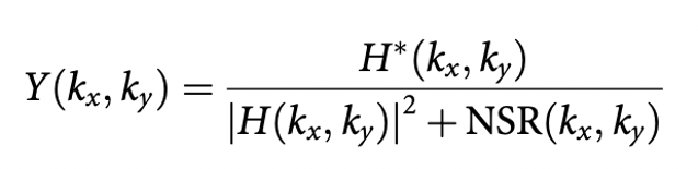
The value of NSR(kx,ky) used in this equation is often approximated as a constant. This constant is generally found by testing multiple values and identifying which yields the best performance, which is the method we chose for this project.
To compute the MTF, we used the slant edge test. The Slanted Edge is a standard method for measuring sharpness in digital imaging. We followed the test described in the International Organization for Standardization (ISO) standard 12233:2014, which provides guidelines for performing the test and interpret- ing the results. ISO 12233:2014 specifies the technical requirements for image sharpness and describes the Slanted Edge method as one of the recommended approaches for measuring sharpness. The Slanted Edge test provides a method to characterize MTF in a spectrum of different frequencies.
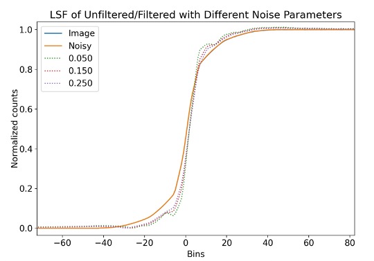
In the Slanted Edge test, a chart with a slanted edge is photographed using the imaging system being tested. The edge is at a 5 degree angle and has a high contrast with the background. The image is then analyzed using an algorithm that calculates the edge spread function (ESF), a profile across the edge, and the line spread function (LSF) is the derivative of the ESF. Taking the Fourier transform of the LSF, we can characterize the response of an optical system in its MTF. The Slanted Edge test was selected for our method to evaluate system performance for being an industry standard with the ability to characterize MTF at a spectrum of spatial frequencies at precise fields.
Method
We used simulations to validate our image sharpening algorithm for a real system. Using optical design software (Zemax), we retrieve phase information of the optical system and simulate images to be tested with our algorithm. From the desired requirements from our customer, we designed a first order system and simulated it with catalog components. A Thorlabs 50X microscope and Thorlabs tube lens was simulated using the manufacturer’s Zemax Black Box files.

Our algorithm requires the use of the point spread function (PSF) of the system. This PSF was obtained from the simulation in a 512 by 512 array. The simulated PSF will have physical dimensions in xˆ and yˆ. This can be system-specific and can also depend on factors like pupil sampling and system specification. Unfortunately, we found that this simulated PSF was sampled differently from the image. We wrote code to adjust the sampling of the PSF in order to accurately compute the deconvolution. We computed the scaling factor to be 2.660.
Testing and Validation
To test our image correction algorithm, we will use simulated images of a slant edge, then use our algorithm to correct this image. We compute the MTF of the image both pre and post correction. We then compare these MTF curves to the diffraction limited MTF to quantify the performance of the algorithm. An example of these MTF calculations are provided below.
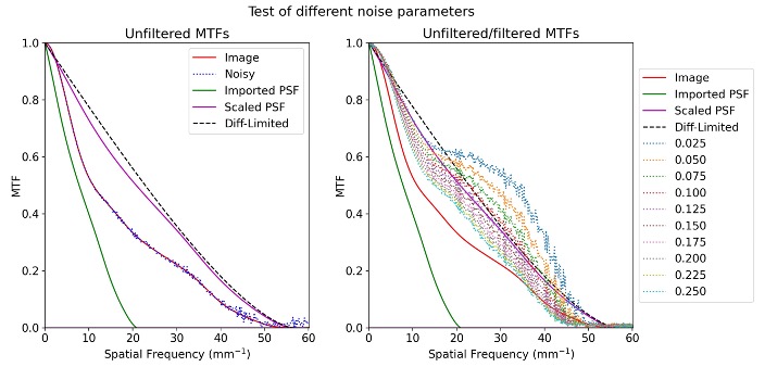
We found that the Wiener Helstrom filter is capable of raising the MTF beyond the diffraction limited value, but at the cost of creating ringing artifacts at edges within the image. As can be seen in Figure 6, a smaller noise coefficient is capable of making the image sharper, but comes at the cost of increased ringing. For the purposes of this project, we decided to optimize the balance between ringing and sharpness to minimize the squared difference between the MTF of the output image and the diffraction limited MTF.
Conclusions
The Wiener Helstrom filter has proven to be capable of improving the MTF to be even better than the diffraction limited MTF, however this comes at the cost of creating ringing artifacts in the image. The noise parameter used in the filter can be chosen to achieve a certain balance the sharpening and the ringing. We chose to identify what value of this parameter minimizes the squared difference between the output MTF and the diffraction limited MTF. The value we found our system was 0.08.
Acknowledgements
We would like to thank our faculty advisor, Dr. Jim Fienup for his invaluable expertise in computational image correction and guidance with the project. We would also like to thank our customer, Dr. Andres Guevara, and our professor, Dr. Wayne H. Knox for their guidance through the year and giving us this project to tackle.