Team
Yihan Shao
Chuqin Wu
Melanie Xue
Zihe Zheng
Mentor
Cantay Çalışkan
Abstract
The goal of this project is to forecast the pest pressure of Grape Powdery Mildew at a specific location to allow growers to treat this plant disease in time. We will experiment with various Time Series Forecasting (Index: 0 to 100) and Classification (classes: Low, Medium, and High) models to predict Grape Powdery Mildew disease pressure in a given area.

1. Background
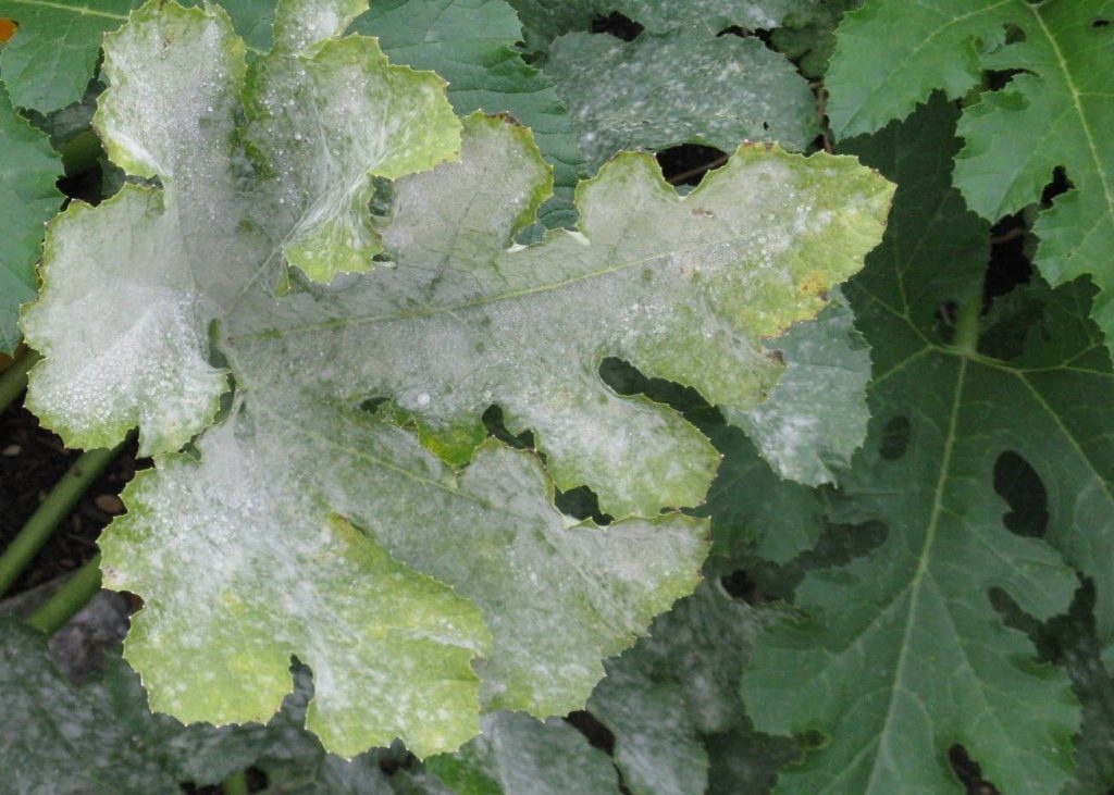
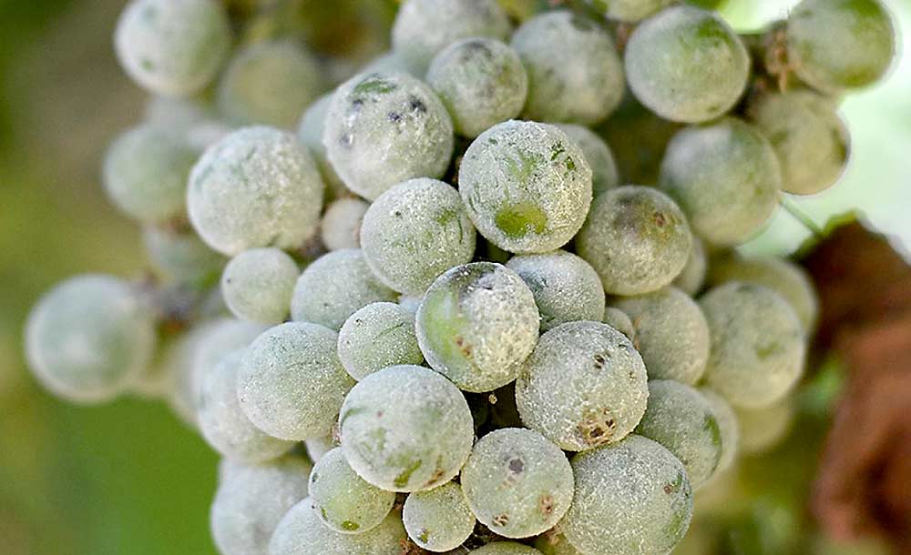
1.1 Powdery Mildew
Powdery Mildew is a type of fungal disease that could happen on many types of plants, and it is crop-specific. In this project, we will be focusing on grape powdery mildew in California. For grapes, powdery mildew will cause the fruit to have bad tastes, and a small portion of the bad grapes will destroy the entire barrel of wine.
Conidial spore production occurs 7 to 10 days after primary infection and conidia will continue to be produced throughout the season as long as moderate temperatures (70° to 85°F) exist. Grape powdery Mildew also likes arid environments, but the temperature is still the primary factor.
The fungus survives the winter inside dormant buds, and then emerging shoots may become diseased shortly after bud break. It is worth noting that the fungus of Powdery Mildew will always exist; thus, our goal is not to find a way to exterminate the fungus but to help with slowing down or stopping its spread. Season-long control of Powdery Mildew is dependent upon reducing early-season inoculum and subsequent infection. Because with fewer initially infected plants, the smaller the potential size of spread would follow. Thus, treatment must begin promptly and be repeated at appropriate intervals.
1.2 Powdery Mildew Index (PMI)
The purpose of the powdery mildew index (PMI) is to determine the disease pressure and to instruct grape growers when and what to use to protect the vines.
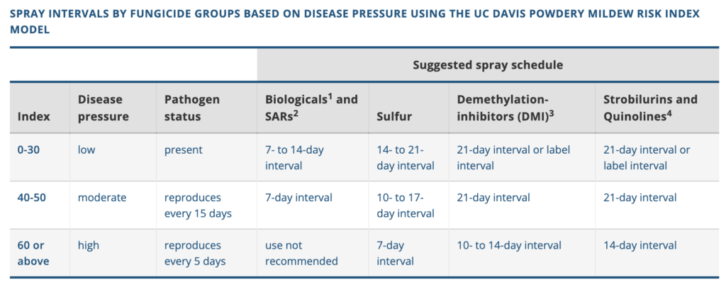
When the calculated PMI is less than 30, the disease pressure is low and the pathogen is not reproducing. PMI between 40 and 50 is considered moderate and the pathogen reproduces every 15 days. PMI above 60 indicates high disease pressure, and the pathogen reproduces every 5 days. There are four common fungicide sprays to protect vines, and the grape growers can choose the appropriate spray schedule based on this table. It is important to alternate fungicides to prevent pathogen populations from developing resistance to classes of fungicides.
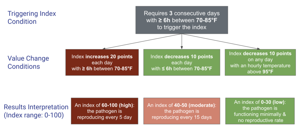
One of the challenges of this project is that we did not have the true observations of power mildew. Instead of having an actual measurement of Powdery Mildew in the field, we only have this calculated PMI, using the PMI model proposed by UC Davis. PMI is calculated purely based on temperature, to theoretically evaluate the powdery mildew pressure in the field.
We follow the steps in the flowchart below to compete for PMI using hourly temperature data. There are to be three consecutive days that have at least six hours of temperature between 70 to 85 Fahrenheit to trigger the PMI. Once triggered, the model will start with a base index of 60. If the index reaches 100, there will be no more addition; and if the index reaches 0, there will be no more subtraction. The output index will range between 0 and 100.
2. Exploratory Data Analysis
2.1 PMI Trends
We have computed the annual PMI trends based on hourly temperature, using the US Davis model above. We can see that most of the high and median PMI risks happen between mid-March and Early-November.
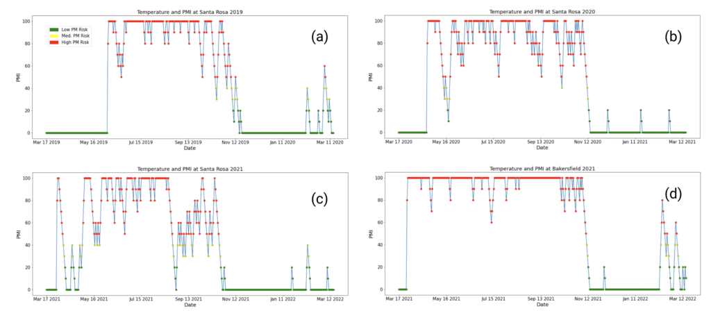
We can observe some patterns from the four plots above. At the same station, although the PMI trend varies over years, there are still some similar trends. For example, in Santa Rosa, both 2020 and 2021 have dips in mid-May; both 2019 and 2020 have dips in mid-October. During the same year, different locations might have different PMI trends. The bottom two plots compare the trends of different locations – Santa Rosa and Bakersfield – in 2021. Even though the extent of PM pressure for both stations are different during the season, most of the high and median PMI risks still happen within the same period.
2.2 ACF & PACF Analysis
To explore the correlation between a given time series and the series with its lagged value, we applied the auto-correlation function (ACF) and partial auto-correlation function (PACF). The Figure blow displays the ACF and PACF results for the hourly and monthly temperature series. From previous visualizations, it could be observed that two series have distinct daily and yearly periodicity, suggesting that they are non-stationary. Since the algorithm requires the input series to be stationary, we first attempted to eliminate seasonality by taking a 24-hour and 12-month difference, respectively, and then applied functions. As can be observed from chart (a), the lags of hourly temperature are not diminishing rapidly enough, showing a decrease rate of exponential. And the PACF have significant lags at the first and twenty-fifth positions. Figure (a) demonstrate that even after taking a difference in series, the hourly data retains trends and a daily periodicity.
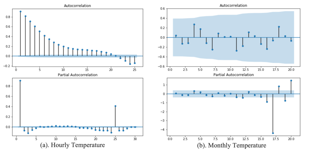
Figure (b) shows the result for monthly temperature. It reveals that all temperature lags fall within the 95% confidence interval (shaded area), indicating that there is no substantial correlation between the present and preceding values. Additionally, it can be seen that the ACF distribution for temperature is comparable to that of a white noise. As a result, it implies that there exists no additional extra pattern or periodicity after eliminating the yearly seasonality.
3. Model Development
3.1 ARIMA
ARIMA is an acronym for Autoregressive (AR) Integrated Moving Average (MA) Model. To demonstrate the algorithm, we selected the area of Poway as an example to illustrate the findings. We experienced two training and testing lengths with testing sets 10 days and 20 days respectively. Considering the powdery mildew grows considerably faster than other seasons, we selected the test set to be in August. The above figure (a). shows the predicted results of hourly temperature and hourly PMI for the model with training set from 04/23/2021 – 07/31/2021 (100 days) and test set from 08/01/2021 – 08/10/2021 (10 days); The bottom figure (b). displays the results for training set from 01/21/2021 – 08/08/2021 (200 days) and test set from 08/09/021 – 08/28/2021 (20 days).
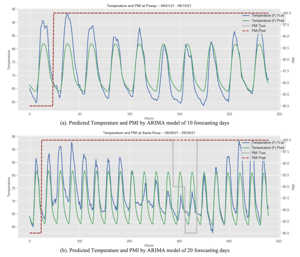
Both graphs demonstrate that ARIMA models are capable of capturing the general trend of hourly temperature, as seen by their accurate prediction of daily periodicity. However, it is also clear that the algorithm is inadequate at identifying daily fluctuations. As the daily average temperature varies within 10 days, the model has lower predictive values for days with a temperature higher than the mean, and vice versa. Additionally, by comparing Figure (a) and (b), we may deduce that the ARIMA model is unsuitable for long-term prediction, since the MSE is 18.295 for 10 days and 33.862 for 20 days, with the latter being almost twice the former. It’s also worth noting that due to the method used to calculate the PMI, the predicted PMI index coincidentally equals the true PMI in 10 days forecasting model.
3.2 LSTM
Long short-term memory (LSTM) (source) is an artificial neural network commonly used in time-series forecasting. Originated from Recurrent Neural Networks (RNN) (source), LSTM has the ability to allow previous outputs to be used as inputs while having hidden states. There are three parts (gates) in a LSTM cell. The forget gate chooses which information from the previous timestamp is to be remembered. The input gate adds or updates new information to learn. The Output gate passes the updated information to the next timestamp. By changing the dimensionality of the input and output space, we can control how many hours/days we use for prediction as well as how many days we want to predict ahead.
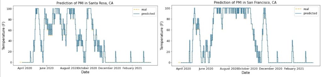
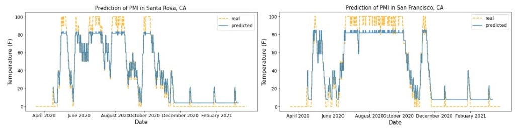
To predict hourley PMI, we trained our LSTM model on the Santa Rosa hourly PMI data during the period of 3/17/2019-3/16/2020. The parameters were set so that the model could predict one hour ahead based on the past 7*24 hours. We trained the model for 500 epochs. To test our model, we used the Santa Rosa hourly PMI during the period of 3/17/2020-3/16/2021, and the San Francisco hourly PMI during the period of 3/17/2020-3/16/2021. The MSE were 4.633 and 3.963 respectively. It can be observed that the real and predicted PMI are very much aligned with each other, which is an improvement of the previous method. The MSE for San Francisco is even lower than the MSE for Santa Rosa even though we only trained on the Santa Rosa data, which means that our model can be generalized for other areas without additional training.
To make our model even more practical, we tried to predict 7 days ahead based on the previous 30 days of hourly PMI. We chose 7 days because the treatments for PMI are usually based on weeks. The training data and procedure was similar to above but due to time limitation, we only trained for 50 epochs. The result shows that the predicted values tend to be more conservative and less spread out than the real values. We believe that this issue can be fixed with more epochs of training since a similar shape of predicted values also appeared at the early stage of training for the one-hour prediction.
4. Conclusion
4.1 Achievements
For time series prediction, our ARIMA model can capture the overall daily trends but may ignore temperature variations (MSE 18.295). It is not suitable for long-term forecasting (MSE 33.862). Our LSTM model can predict PMI directly based on the past 7 days at an MSE of 4.633. It is also feasible to predict 7 days ahead using the hourly PMI of the past 30 days. Our model can easily generalize to other areas, which saves time for repeated model training.
For the classification of PMI levels, both Random Forest and Gradient Boosting achieved an accuracy of 75%. Random Forest has a more stable prediction performance than Gradient Boosting.
To conclude, Our time series models can accurately predict PMI with precision in hours and have the potential to be used in real-life applications. Our classification models are more time-efficient and can provide real-time predictions of PMI class based on climate data.
4.2 Future Work
In the future, if a suitable amount of true observations of grape powdery mildew in the field are avalivable, we will be able to better our current model by using gound-true values of the powdery mildew variable. In addition, since the predicting variable is no longer a non-linear representation of hourly temperature, we will also be able to include more agriculture-related features when constructing new models.