Team
- Jike Lu
- Mingjun Ma
- Jiayue Meng
- Zheng Tong
Academic Advisor
Prof. Ajay Anand and Prof. Cantay Caliskan
Project Sponsor
Dr. Erika Ramsdale and the URMC Geriatric Oncology Team
Introduction
Studies in recent years have shown that cancer rates have declined in the overall population, but are on the rise in people over the age of 65. In fact, people over 65 years old are about 11 times more likely to develop cancer than people under 65 years old[1]. Therefore, cancer treatment for the elderly has been a topic of widespread interest in the medical field. However, many approaches to cancer treatment are accompanied by serious side effects, such as pain, or frequent falls[2]. On the other hand, older adults with advanced cancer are often accompanied by many other health problems, such as cognitive challenges, heart disease, and diabetes, among other health conditions[2]. In this context, the question of how to reduce the side effects of treatment in older adults with advanced cancer is an urgent one that deserves research. To address this issue, the results of a clinical trial suggest that a health measurement tool called geriatric assessment can play a key role in reducing serious side effects during cancer treatment. In this study, clinic staff can make adjustments to a patient’s treatment plan based on the results of geriatric assessments, such as reducing the intensity of a patient’s treatment or enhancing supportive care[2].
In this context, the Geriatric Oncology group from the University of Rochester Medical Center (URMC) wanted to analyze the results of geriatric assessments of patients at a certain point in time to predict patients’ tolerance to side effects of cancer treatment in the following period and to make timely adjustments to the treatment plan. During this semester, our team collaborated with the URMC Geriatric Oncology Group to investigate this project through the lens of data science. By studying this project, we intend to help clinicians have a better understanding of the data they collected, on the basis of which we want to predict how well patients will tolerate the side effects of subsequent treatments based on data from a certain period of time. Also, we want to determine what the most appropriate time interval is between each geriatric assessment. In addition, we wish to find the features that have the greatest impact on the prediction results.
Dataset
Dataset Description
The URMC Geriatric Oncology Group collected data from 737 patients about the results of the geriatric assessments. The data contains the results of four geriatric assessments for each patient over a six-month period, which are screening, 4-6 week follow-up, 3-month follow-up, and 6-month follow-up. The URMC Geriatric Oncology group also collected many other pieces of information in detail, such as the patient’s personal information, the patient’s physical indicators, and the patient’s treating physician’s information. The complete dataset contains a total of 2,948 rows and 1,056 columns of data. However, many of the features are not relevant to the topic of our study. After discussion with the URMC Geriatric Oncology group, 138 variables that related to the direction of our study were selected from the original dataset. These 138 variables can be grouped into five categories based on their nature:
- Demographical Data including information about the patient’s ID, assessment stage, gender, age, education, marital status, living situation, and income situation.
- Cancer & Treatment Type Data including information about the patient’s cancer type and the treatment type they received.
- Health Status Indicators including the results of various tests performed on the patient’s health status, such as the timed up & go (TUG) test score, activities of daily living (ADL) score, the Geriatric Depression Scale (GDS), etc.
- Symptoms including 28 symptoms recorded by geriatric assessment, such as pain, vomiting, dizziness, etc.
Our outcome variable pertains to whether chemotherapy’s side effects align with patients’ expectations.
Data Preprocessing
Given the considerable number of missing values in our dataset, it is crucial to handle them with caution. Initially, we attempted to impute the NaN values using two prevalent methods: eliminating them or substituting them with the mean values of the respective features. Unfortunately, both of these methods did not yield satisfactory results and failed to align with our objectives. The primary reason for the unsatisfactory outcomes is that removing all NaN values results in a significant reduction in the size of our training set. Moreover, since our data contains a substantial number of missing values, replacing them with the mean value underestimates the variability of the dataset.
Our initial failure attempt prompted us to explore other imputation techniques, and we ultimately settled on imputing missing values based on the functions of other variables. However, since our dataset contained over a hundred features, and most of them were not linearly correlated, the traditional multivariate feature imputation method was not feasible. Consequently, we decided to adopt the nearest neighbor imputation method, which entailed imputing missing values based on the Euclidean distance of variables.
Given that we were predicting an emotional outcome, we aimed to minimize the variability of the outcome variable as much as possible. Therefore, we binarized our outcome variable to enhance the practicality of our results. Instead of multiple levels of satisfaction, we made a binary variable that categorized patients as either satisfied or unsatisfied with their treatment based on whether they thought the treatment met their expectations. Specifically, we assigned patients with an outcome variable of less than 3 as those who felt that the treatment did not meet their expectations, while patients with an outcome variable of 3 or higher were considered to have felt that the treatment met or exceeded their expectations.
Exploratory Data Analysis
After examining the demographic variables, we found that the number of male patients was more significant than that of female patients. Also, most patients are non-Hispanic white people. The analysis of age groups reveals that most patients are in the age group of 70–79, and most of them have at least a high school degree. Furthermore, most patients get married and live with someone instead of being alone. By checking their income, we find that most earn an annual income of less than $50,000.
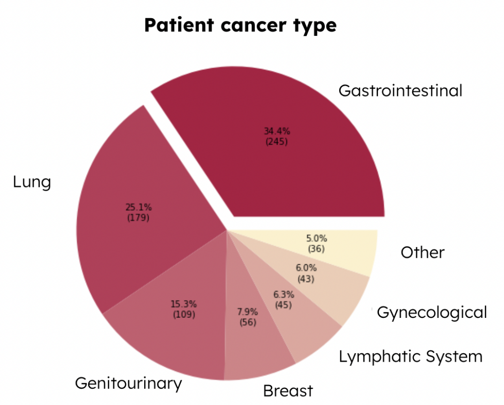
Then we checked the variable of cancer type, which is a categorical variable, indicating 6 types of major cancer, and the rest of the types of cancer are classified as “Other.” This cancer type pie chart below presents the distribution of each type of cancer among patients (Figure 1). We can see that the most common type is gastrointestinal cancer, which takes up around 34.4\% of the total patients, and the second most common type is lung cancer, which takes up to 25.1\% of the total patients. Since different types of cancer require different treatments, it is also important to understand the variables related to the types of treatments.
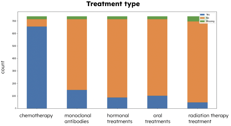
Types of treatments are another significant categorical variable that indicates the distribution of applications of different types of treatments. From the Treatment Type stacked bar chart (Figure 2), we can see that there are 5 types of treatment: chemotherapy, monoclonal antibodies, hormonal treatments, oral treatments, and radiation therapy treatment. From the chart, we noticed that most patients received chemotherapy. Cancer treatments would induce various symptoms in patients, so it is crucial to understand some trends in the symptoms variables.
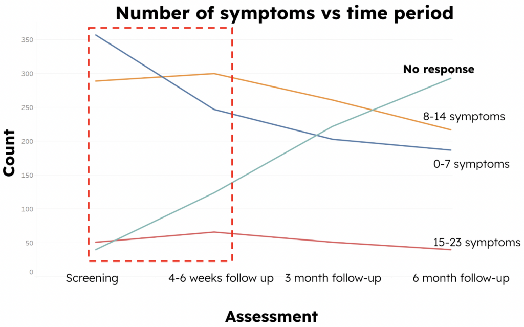
To further analyze the trend in the number of patient symptoms over time, we created a line chart of change in symptoms (Figure 3), and we can see that the number of non-responders is increasing in each assessment period. However, from the screening period to the 4-6 week follow-up period, as shown in the red frame, we could find that the number of patients who have 0-7 symptoms is decreasing, whereas the number of patients who have more than 7 symptoms is increasing. This indicates an overall upward trend in the number of patient symptoms.
Model Development & Performance
Feature Selection
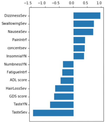
Figure 4 displays the outcome of our feature selection process, where we utilized Lasso regression with a threshold of 0.3. As illustrated, important symptoms such as dizziness, swallowing, and taste had the highest absolute values of coefficients. These symptoms were then employed as input in our classification models, resulting in a good ROC curve and accuracy when compared to using all features simultaneously.
Classification Models
We tried five popular classification models in total: logistic regression, random forest, support vector machine, Naive Bayes, and long short-term memory networks. After careful consideration, we decided to finally use SVM for several reasons that will be covered in the following sections. In addition, we concluded that 3 months is the optimal duration for administering chemotherapy before assessing if there is a regression because models trained by the data in the third month not only give us high accuracy but also give certain time intervals for clinicians’ interventions. If we use data from one assessment period to predict patients’ feedback at that period, clinicians don’t have time to intervene and adjust their treatments based on our predictions. If we use data from 4 to 6 weeks to predict their feedback in the sixth month, the accuracies and AUC values are undesirable. So, we determined that using assessment data in the third month was the best option.
Logistic Regression
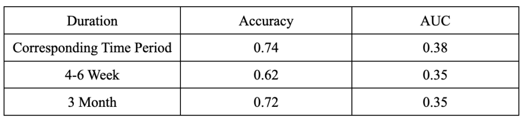
In our project, logistic regression didn’t give a good performance as its AUC values were under 0.5 for all durations, meaning that the prediction results were not better than random guessing (Figure 5).
Random Forest
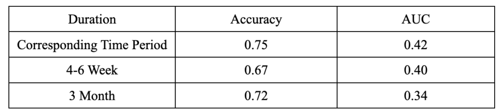
We can see from the table below (Figure 6) that random forest has poor performance on the AUC for all durations, despite its relatively high accuracy at a 3-month duration.
Naive Bayes
In our project, Naive Bayes had unsatisfactory performances compared to other models. It produced low accuracies and AUC at all durations. Thus, we decided not to further analyze it in detail.
Support Vector Machine (SVM)
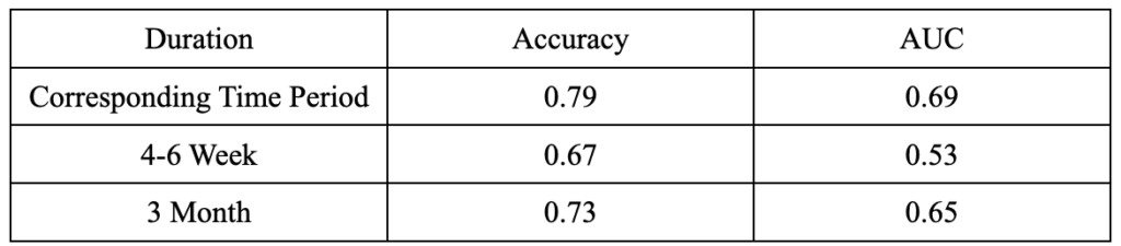
In the project, SVM generated both good accuracies and AUC values (Figure 7). When we used assessment data in the third month to predict results in the sixth month, SVM had an accuracy of 0.73 and an AUC of 0.65, which are satisfactory results considering we are predicting an emotional variable (patients’ expectations) using clinical data. When we used assessment data at each period to predict results at that corresponding time period, we got even better results: an accuracy of 0.79 and an AUC of 0.69. However, due to the reasons explained in 4.3, we still decided to use the SVM model using the data in the third month.
Neural Networks: Long Short-Term Memory Networks (LSTM)
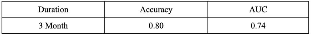
The LSTM (Long Short-Term Memory) model is a type of recurrent neural network (RNN) used in machine learning. Since we determined that 3 months is the optimal duration, we tried the LSTM model on our dataset. It has a performance score of 0.80 and an AUC of 0.74 (Figure 8).
However, it is not the optimal model for our project, and we still decided to use the SVM model for two reasons. Firstly, Long short-term memory networks used 143 features, which is much more than physicians and clinicians would use in reality. If we have a huge amount of features in a dataset, Long short-term memory networks might require a large amount of time to train. So, even if it has the best performance, it is not practical in reality. In comparison, SVM used only 13 features to reach a good accuracy of 0.73 and an AUC of 0.69, so it is more manageable and practical in the field of clinical medicine. Secondly, SVM has better explainability. It is hard to explain why and how certain features contribute to the prediction in neural network models because of the models’ non-linearity, high dimensionality, complex internal structures, and lack of interpretability. It is difficult to isolate individual feature contributions in neural network models because they capture relationships and interactions between features. Additionally, the high dimensionality of the data and the complexity of the networks further complicate interpretability. Also, neural networks are often referred to as “black box” models because they lack explicit interpretability. The models can provide accurate predictions, but the internal mechanisms and decision-making process make it difficult to explain the exact reasons why certain features contribute to the predictions. Although there is some ongoing research about explaining feature contributions in neural networks, it is still a complex and challenging task, especially in the clinical medicine field. Interpretability of clinical models is as important as predictive results because understanding the model’s decision-making process will build trust and transparency among clinicians, patients, and other stakeholders. Also, interpretability makes error detection and improvement possible. Only if people understand the logic behind the models can they test for clinical validation and adoption. In conclusion, interpretability enhances accountability, supports decision-making, and promotes the acceptance and understanding of clinical models within the medical community.
Summary
Logistic regression, random forest, and Naive Bayes models produced unsatisfactory results in terms of accuracy and AUC compared to our SVM and LSTM models. LSTM has the best performance, but due to its practicability and interpretability, we eventually opted to use the SVM model as our best model.
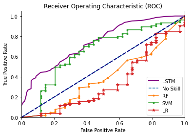
Performance
As shown in Figure 10, we can see that both the LSTM and SVM performed well under the case using the data from the 3-month follow-up to predict patients’ tolerability of cancer treatment during the time until the 6-month follow-up. Although the ROC of the LSTM is 0.74, which is higher than the SVM’s 0.65, it is worth noting that the LSTM uses all 143 variables as input, making it difficult to determine which variables have a more significant impact on the predicted outcome. To be able to provide more advice to clinicians rather than just being limited to better model performance, we decided to use SVM as our final model.
As a result, we suggested clinicians should perform geriatric assessment and record data every three months to make timely and accurate treatment plan adjustments in response to patients.
Conclusion & Future Work
During the research process of the project, we had frequent communication with the research team about the progress and results and came up with many valuable insights.
First, we found that the number of data points was decreasing regularly over time, so we determined that the data were not missing at random. The reason for missing data may be that the patient dropped out of treatment for some reason, or unfortunately passed away during the treatment. In addition, we observed an overall upward trend in the number of symptoms in patients, especially in the first 4-6 weeks of their initial treatment, despite the fact that they were receiving treatment. In fact, studies from the Centers for Disease Control and Prevention have shown that patients have many reactions when they first start cancer treatment, such as Hair Loss, Nausea and Vomiting, Problems with Thinking and Remembering Things, and several pains[3]. In addition, after comparing different feature selection methods, we identified several features that have a strong association with the impact on the prediction results. In order for clinicians to provide patients with timely supportive care to reduce the suffering caused by side effects of cancer treatment, clinicians should focus on whether patients have swallowing issues, dizziness, insomnia, taste issues, nausea, or severe pain; clinicians should also focus on the Geriatric Depression Scale (GDS) and Activities of Daily Living (ADL) score of patients. In order for the clinicians to make the most accurate and timely adjustments to the treatment plan based on patient feedback, they should provide a geriatric assessment for each patient every 3 months.
There are some potential areas for improvement based on the research we have completed so far. In the process of feature selection, we manually filtered out 68 variables from the initial 1,056 features, so there may be some bias in this process. In future work, we can try different data filters manually or using algorithms to reduce the bias. On the other hand, we want to apply our findings to a broader context. Therefore, we aim to increase the external validity of our research so that our models and results could be used for other similar studies.