Team Members
- Kendall Smith
- Madeleine LaChance
- Lukas Ladas
- Marcelo Rocas
Customer
Daniel Brooks – Optimax Systems, Inc.
Mentor
Dr. Aaron Bauer – Institute of Optics
Abstract
The goal of this design project was to build an alignment tool to aid the engineers at Optimax during the alignment process of a freeform reflective triplet system designed by Team CubeSat 2023. This system was designed for use in a cube satellite with the application of analyzing the chemical composition of ice sheets while tracking their size and movement throughout time. Due to the design constraints, the members of Team CubeSat 2023 decided to use freeform surfaces in their design. Freeform surfaces lack translational and rotational symmetry, which introduces additional degrees of freedom not present in traditional spherical surfaces. Systems with freeform surfaces can utilize these degrees of freedom for many different applications, including miniaturization of the system and a reduced number of components, but they can be very difficult to align as compared to spherical systems because the additional degrees of freedom can result in very complex wavefront errors. It is therefore nearly impossible to determine which surface is misaligned and what adjustments need to be made to properly align a freeform system by simply looking at an interferogram output from the system. This alignment tool will solve this problem by calculating the Zernike coefficients from an interferogram of the misaligned system and inputting them into a least squares algorithm to determine the adjustments which need to be made to better align the system.
Current Design
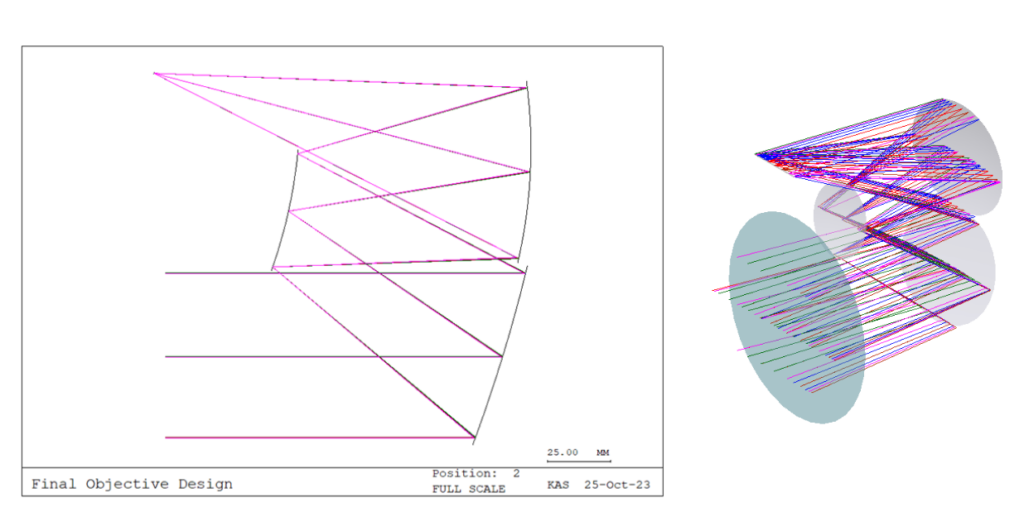
The design completed by last year’s CubeSat team consisted of three freeform reflective surfaces. All mirrors were fitted using 37 fringe Zernike coefficients in the CodeV environment. A drawing of their design in CodeV is shown below. This design served as the starting point for our tolerancing analyses, and we used it to build our alignment tool.
Alignment Tool
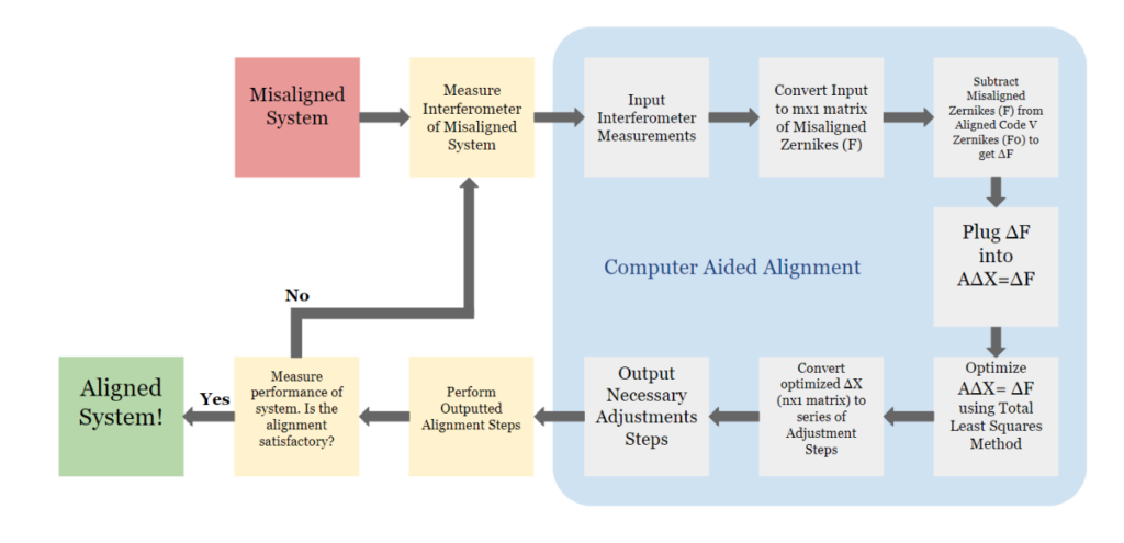
The figure above illustrates how our alignment tool will be incorporated into the alignment process at Optimax. The technicians will align the system within the given tolerances and will obtain an interferogram from the misaligned system. This interferogram will be input into our tool, which carries out all the operations contained in the blue box. First, the tool will calculate the first 16 fringe Zernike coefficients from the interferogram measurement and convert the calculated values to a 16 x 1 matrix, where each row is one Zernike coefficient. The remaining steps comprise the least squares algorithm, which will be discussed in more detail in a following section. The algorithm outputs the adjustments which will best correct the system. The technician will then perform these adjustments and use an interferogram measurement to determine if the system is sufficiently aligned. If so, the process is complete. If not, the interferogram will be input into the tool again, and the process will repeat iteratively until the system is sufficiently aligned.
Lookup Table
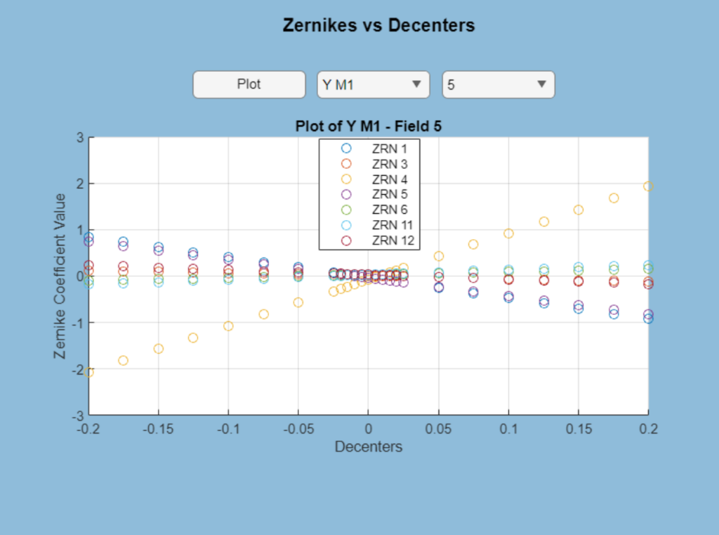
In order to analyze how the Zernike coefficients change with each alignment error, we built a lookup table which can be used by the engineers at Optimax when they are aligning the system. We built a buffer which perturbs both the decenters and tilts of each of the mirrors one at a time. For the decenters, we perturbed the mirrors by increments of 25 microns from -200 microns to +200 microns in the x, y, and z directions and recorded the first 36 fringe Zernike coefficients from each perturbation at 5 different fields. As for the tilts, we perturbed the alpha, beta, and gamma tilts of the mirrors by increments of 0.025 degrees from -0.2 degrees to 0.2 degrees and followed the same process for recording the Zernike coefficients. The data we extracted from this procedure provided useful information on the aberrations generated by each misalignment, which was used later on in our least squares algorithm. We also included it in our GUI for reference; the engineers can choose which mirror, misalignment, and field they would like to examine further, and our GUI will pull up the corresponding graphs of Zernike coefficients versus misalignment. An example is given below; it shows the seven most severe Zernike coefficients through perturbation of the y decenter for Mirror 1, Field 5.
Compensators
In addition to the data in our lookup table, before building our least squares algorithm, we needed to determine what the best compensators would be for our system. Traditionally, in reflective systems, the secondary mirror is used as the compensator during alignment because it is usually the smallest mirror, so it is the easiest to adjust. Ideally, only one mirror is used as a compensator for practical reasons, with all the degrees of freedom enabled (i.e. XYZ decenter as well as alpha, beta, and gamma tilt). However, if the system is sensitive enough, limited degrees of freedom can be enabled on additional surfaces.
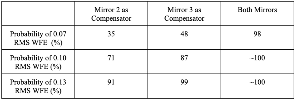
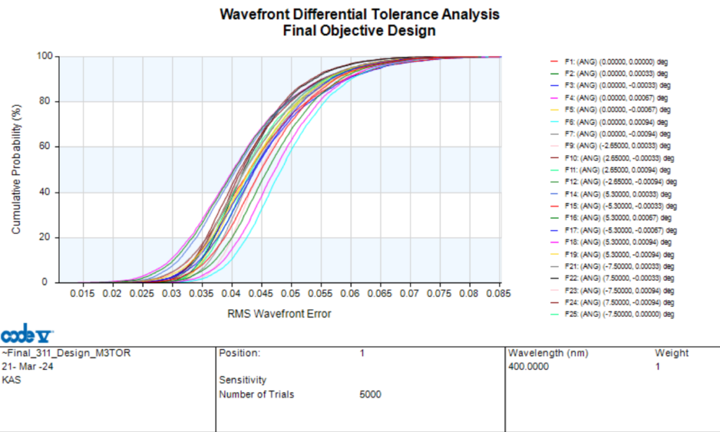
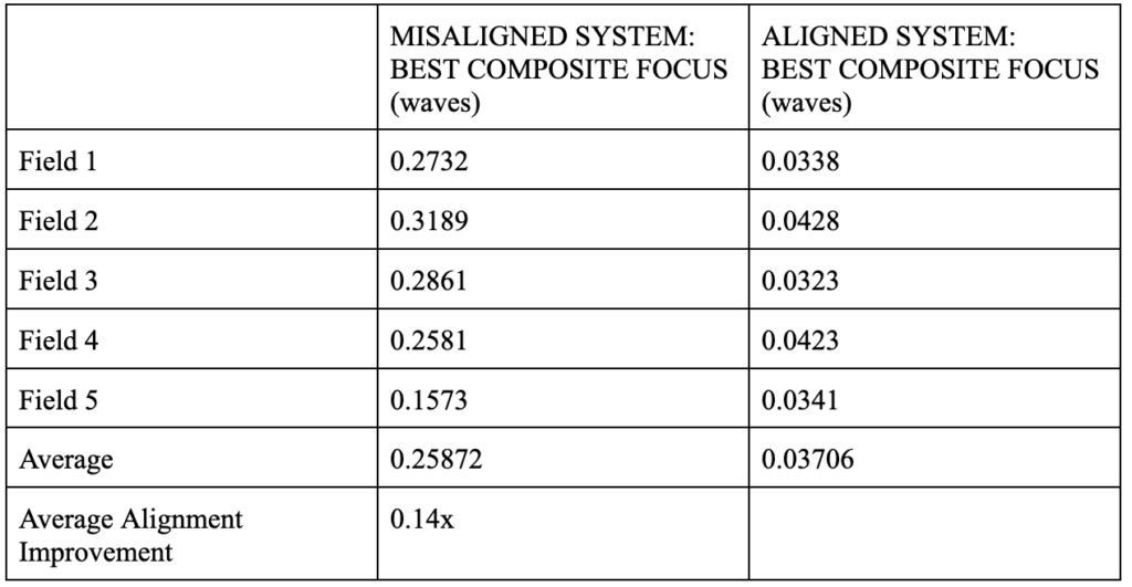
In order to determine which mirror would serve as the best compensator in our system, we ran a TOR analysis in CodeV to determine the most sensitive surface in our system. From this analysis, we determine that Mirror 3 is the most sensitive surface, so it makes the most sense to use Mirror 3 as the compensator. However, Mirror 2 was also rather sensitive, and since Mirror 2 is traditionally used as the compensator, we tried to determine if we could align the system sufficiently using just Mirror 2 as the compensator. We ran three separate Monte Carlo tolerance analysis: one with Mirror 2 as the compensator, one with Mirror 3 as the compensator, and one with both Mirror 2 and Mirror 3 as compensators, with limited degrees of freedom enables on Mirror 3. A table of the results is shown below, as well as an image of the output from the Monte Carlo analysis using both Mirror 2 and Mirror 3 as compensators. As can be seen from the table, it is best if we use both Mirror 2 and Mirror 3 as compensators.
Least Squares Algorithm
With our Lookup Table completed and our compensators determined, we had enough information to build the least squares optimization algorithm. This algorithm took two matrices as its inputs. The first matrix was a Sensitivity Matrix; each value in this matrix is the partial derivative of the change in Zernike coefficients with respect to a specific alignment error. The second matrix was a matrix of the difference between the Zernike coefficients of the aligned system and the Zernike coefficients of the misaligned system. These matrices were input into a least squares optimization function in Matlab, and the function output a matrix of the adjustments which need to be made to better align the system.
Simulation
To ensure that our alignment tool was working correctly, we ran a simulation with our model in CodeV. We first manually added random perturbations to each surface in CodeV. We then input the Zernike coefficients of this misaligned system into the least squares optimization function in Matlab. The function yielded a matrix of recommended adjustments, which we manually added to each surface in CodeV. After adjusting the model in CodeV, we recorded how much the performance of the system improved. The results are shown in Table 2. Our alignment tool successfully improved the performance of the system by a factor of 0.14X. However, the least squares optimization function only converged when very small perturbations were added to each surface. We determined that our alignment tool is only able to handle decenters of ±10 μm on each surface, and tilts of ± 0.01°. These tolerances are very tight, but they are not atypical of freeform reflective systems, so this result is not overly concerning.
Zernike Extraction
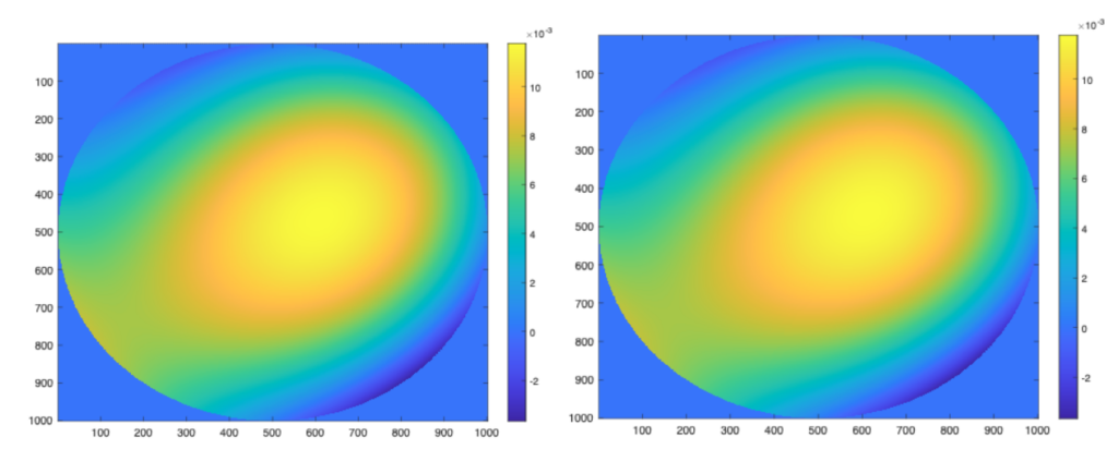
Although we ran the simulation using Zernike coefficients from CodeV, our alignment tool is also capable of extracting the Zernike coefficients from an interferogram. In reality, when the engineers are aligning the system, they will not have the Zernike coefficients of the misaligned system; all they will have is an interferogram. Our code fits an interferogram to the first 16 fringe Zernike coefficients. We didn’t fit to the higher Zernike coefficients because these correspond to higher order aberrations which almost always have a value of zero. Figure 5 illustrates a sample interferogram on the left and the fitted wavefront from our code on the right. As can be seen from this figure, our code sufficiently fits a given wavefront to 16 fringe Zernike coefficients, which can then be input into the least squares optimization function.
Conclusion
In conclusion, we successfully built an alignment tool using a least squares optimization function. This tool is capable of aligning the freeform reflective system designed by Team CubeSat within the desired specification for RMS wavefront error, provided that the mirrors are aligned within ±10 μm in the x, y, and z directions and within ± 0.01° in the alpha, beta, and gamma tilt directions. These tolerances are very tight, but Optimax has tools capable of aligning the mirrors within these tolerances.
Acknowledgements
We would like to thank our advisor, Dr. Aaron Bauer, for all his advice on modeling freeform surfaces in CodeV and for catching all of our many mistakes. We would also like to thank our customer, Dan Brooks, for his help throughout the design process. The insight and information he provided regarding the manufacture of freeform surfaces was invaluable. Finally, we would like to thank Professor Wayne Knox for his guidance throughout the course of this project.
Primary References
- E.P. Goodwin and J.C. Wyant. “Zernike Polynomials”. Field Guide to Interferometric Optical Testing, SPIE Press, Bellingham, WA, 2006.
- Jide Zhou, Jun Chang, Guijuan Xie, and Ke Zhang “Study on computer-aided alignment method of reflective zoom systems”, Proc. SPIE 9618, 2015 International Conference on Optical Instruments and Technology: Optical Systems and Modern Optoelectronic Instruments, 96180L (5 August 2015); https://doi.org/10.1117/12.2190073.
- Kruschwitz B. “Module 2: Intro to Interferometry and Optical Testing.” OPT 242 Aberrations, Interferometry, and Optical Testing, The Institute of Optics, University of Rochester. 2023, pg. 26.
- Margalit, Dan and Rabinoff, Joseph. “ The Method of Least Squares.” Georgia Institute of Technology: Interactive Linear Algebra. https://textbooks.math.gatech.edu/ila/least-squares.html.
- Niu, Kuo and Chao Tian. “Zernike polynomials and their applications.” Journal of Optics, vol. 24, no. 12, 15 November 2022. DOI 10.1088/2040-8986/ac9e08.
- “What is Freeform Optics?” Center for Freeform Optics, http://centerfreeformoptics.org/what-is-freeform-optics/. Accessed 1 November 2023.