Modeling of Lake St. Louis Water Levels

Authors:

Guanjie Linghu

Data Science | Mathematics | Business | ’21

Xiaobo Luo

Ling Liu

Francisco Ambrosini

Data Science | Economics | ’21

Sung Beom Park

Data Science | Mathematics | ’21

Supervisors

• Ajay Anand
• Pedro Fernandez
• Department of Data Science at the University of Rochester

Sponsors

• Bernie Gigas
• David Fay

Background

Lake Ontario set record water levels in 2017 and 2019. The general population that resides around Lake Ontario does not have easy access to relevant system data and analysis. Although regulatory agencies have internal correlations, little to none is available in the public domain. This is where our team and I come in and develop a model that will accurately predict St. Louis Lake water level at any given time.

Goal

The main objective is to identify the maximum water flow tolerance of the Moses-Saunders Dam in order not to exceed the permissible limits of Lake St. Louis.

Methodologies

1. Clean the provided data and deal with missing values.
2. Exploratory Data Analysis.
3. Build a predictive model based on the provided hydrology information that predicts the water level of St. Louis Lake.
4. Use the above model to calculate or build a new model to predict the maximum water flow tolerance of the Moses-Saunders Dam.

Data Preprocessing

The dataset contained null/missing values. These rows were removed.

Exploratory Data Analysis

• Create correlation and plot heat map to visualize the correlation between each feature.
• Plot the important features to visualize the pattern.

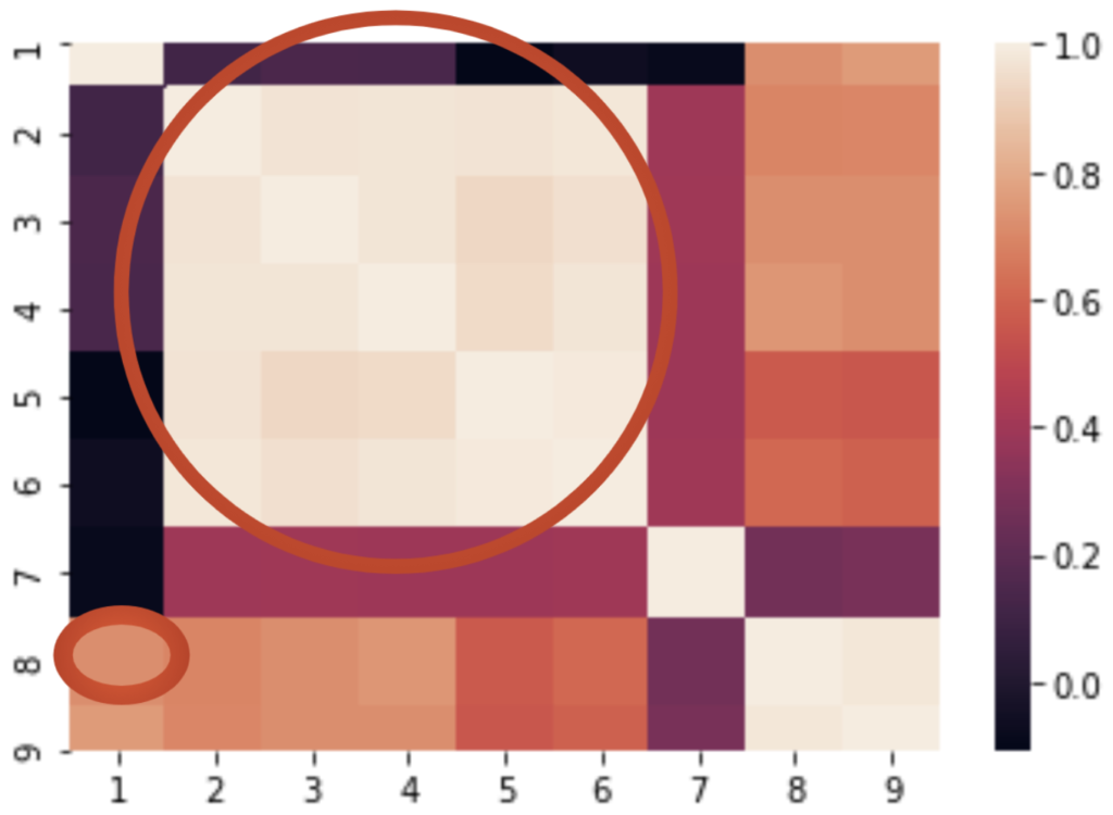
The correlation matrix is visualized as a heat map. The color signifies the amount of correlation.

• Lighter the color, the higher the correlation

• Darker the color, the lower the correlation

The big red circle you see represents areas of extremely high correlation between several rivers and Channel flows. 

The small red oval on the bottom left shows the correlation between the two most important features: The Outflow of Lake Ontario and the water level of Lake St. Louis.

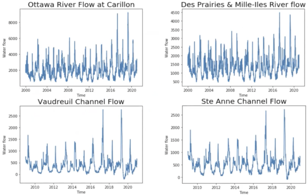
The plot of highly correlated rivers and channels.

We can see very strong seasonal patterns and the difference between the peaks and the medians are extremely large.

These rivers have a strong seasonal overflow problem.

Model development

1. Descriptive model
2. Predictive model
3. Feature importance analysis model
4. Physical long term model
5. Physical short term model

Elastic Net：Base of first three models.

• Pursue high accuracy on numerical result
• Use all input features

Model performance:

Score	open water	Open water and above 22
Max Error (m)	0.22	0.073
Mean Absolute Error (m)	0.024	0.020
Median Absolute Error (m)	0.018	0.016
Root Mean Squared Error (m)	0.033	0.026

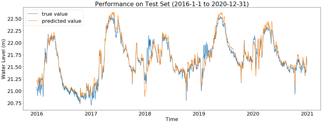
Predictive model

• Obtain a better grasp on practical meaning
• Use all input features except St. Louis Outflow

Model performance:

Score	open water	Open water and above 22
Max Error (m)	0.232	0.176
Mean Absolute Error (m)	0.058	0.042
Median Absolute Error (m)	0.042	0.037
Root Mean Squared Error (m)	0.087	0.050

Feature importance analysis model

• Reduce input dimension while maintain relatively high accuracy
• Only use the “independent” features 
• Use Lake Ontario Outflow, Ottawa River flow, and Chateauguay River flow as input features

Model performance:

Score	open water	Open water and above 22
Max Error (m)	0.358	0.231
Mean Absolute Error (m)	0.054	0.075
Median Absolute Error (m)	0.048	0.073
Root Mean Squared Error (m)	0.067	0.085

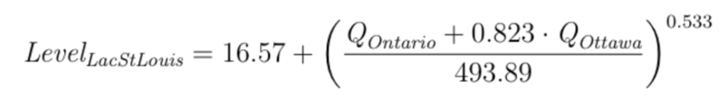
Physical Long term Model

• Want a more physical meaningful model
• Incorporate Chateauguay River flow 
• Divide the open water period into 3 sub periods

Model formula:

Model performance:

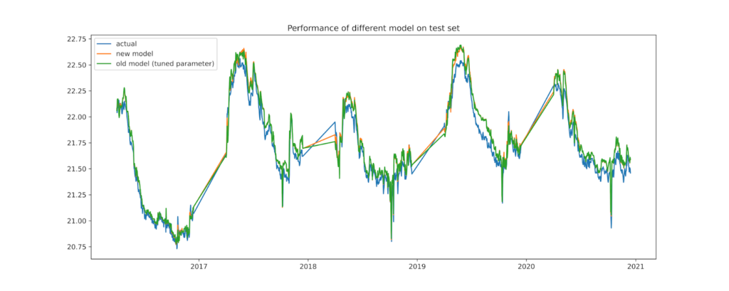
Score	open water	Open water and above 22
Max Error (m)	0.311	0.272
Mean Absolute Error (m)	0.082	0.102
Median Absolute Error (m)	0.077	0.102
Root Mean Squared Error (m)	0.097	0.114

Physical Short term Model 

• Dynamic coefficient in front of Ottawa River
• Use historical St. Louis level to estimate the coefficient
• Use generalized Sigmoid function

Model performance:

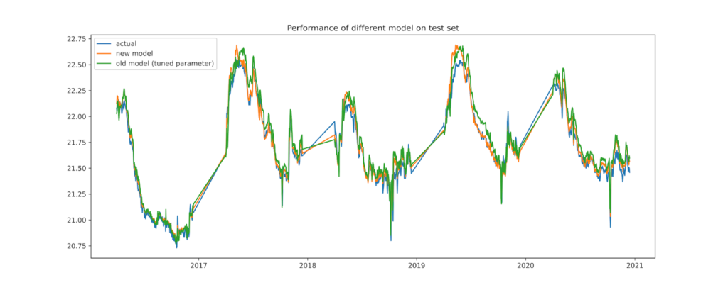
Score	open water	Open water and above 22
Max Error (m)	0.326	0.326
Mean Absolute Error (m)	0.051	0.076
Median Absolute Error (m)	0.037	0.061
Root Mean Squared Error (m)	0.069	0.098

Summary

• Accuracy
  • Descriptive > Predictive > Model 3 > Physical Short Term > Physical Long term
• Trade off between accuracy and physical meaning
• Physical Short Term Model is a “balanced” model with “moderate” performance and high interpretability