Team
- Margaret S Flaum
- Garrett J Percevault
- Adam Smith
Mentor
Thomas Chrien
Abstract
Vision
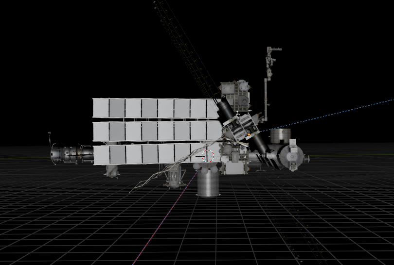
Our goal is to use existing tools and our optical knowledge to build a simulation tool that carries out a rigorous optical analysis and simulates the imaging of a satellite at a range of distances, attitudes, and illumination angles. The simulation tool will import CAD models of various geometries for analysis. The end goal for Millenium Space is to identify satellite images using machine learning algorithms using the fewest number of resolved pixels possible. Therefore, the ability to produce images of various resolutions is of particular interest.
Background


Due to the complex nature of the shape of satellites, for objects more complicated than a sphere, we transitioned to using Blender, a CAD software. Blender provides a simulated image of our satellite with a relative illumination (grayscale) in 8 bits. Our camera is 12 bits, so we needed to then convert this value to what our real grayscale value would be.
Specifications
- Use radiometry to quantify light reflected off a satellite that will be detected by camera in space.
- Produce images of varying resolution from simulation.
- Import 3D CAD Models into Blender
- Include surface properties that are realistic to satellites, by including a combination of diffuse and specular reflection.
- Input the following parameters into Blender:
- Pixel size on CCD
- Number of pixels on CCD
- Camera lens focal length
- Distance between camera and satellite
- Size and shape of satellite/CAD model
- Solar phase angle
- Object surface reflectivity properties
- Input the following parameters into Python:
- Photon Flux per pixel per second (Appendix 3)
- Blender Relative Grayscale Value
- CMOS Quantum Efficiency
- Solar Irradiance
- Pixel pitch
- Satellite Distance
- Focal Length
- Aperture Diameter
- Photons to Grayscale Conversion Factor (Appendix 4)
- Gain
- Well Capacity
- Responsivity
- Expected Noise Equations, based on (Appendix 5)
- Dark Current
- Read Noise
- Grayscale Value
- Exposure time
- Photon Flux per pixel per second (Appendix 3)
- Generate a library of example simulated images of satellites.
Sample Images


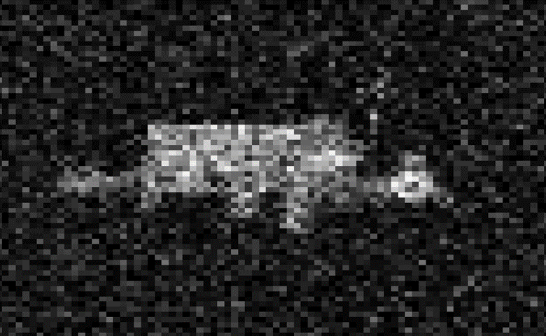
Figure 5: Sample images of the International Space Station at 1000m (top left), 3000m (top right), and 10,000m (bottom)
Calculations
Photon Flux per Pixel
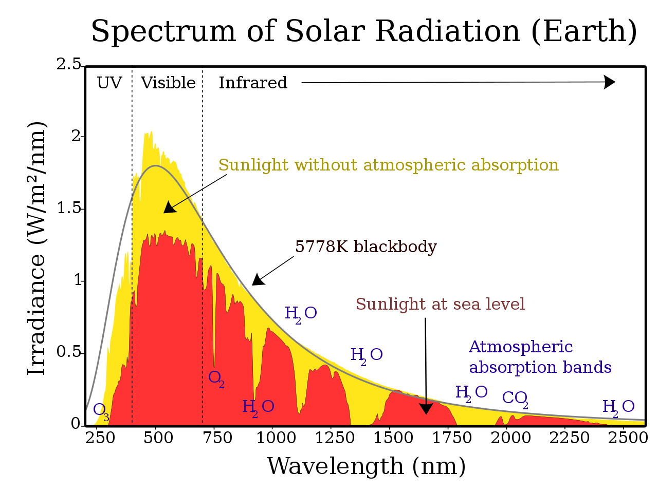
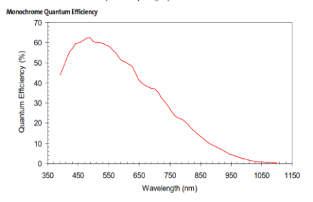
To calculate the expected photons that can be detected by our camera we would integrate the product of the solar spectrum times the quantum efficiency of the detector divided by the energy of a photon.The wavelength range of interest for cameras of this application is 400-1000 nm.

Now, we need to account for the fact not every photon that reaches the satellite will reach our detector.
Flux Per Pixel
This calculation must be expressed per pixel, as each pixel will have a different grayscale value. Therefore, we should calculate the area one pixel will cover at the satellite distance.
Ratio of Photons at Satellite to Photons that reach Camera
We need to find what ratio of total photons emitted from each pixel our sensor will measure. First, we need to define our pixel area, since the calculation will be done on a per pixel basis.

x = satellite distance
f = focal length
We will start by calculating the photon flux for a pixel with the simplest case. We will assume each pixel on the satellite is a flat Lambertian surface that emits photons equally in all directions (half sphere). Furthermore, we will assume the surface that is recorded by pixel is flat to the camera so we will not have to account for any cosine dependence in the calculation.

In this simple example, the amount of photons that will reach the camera lens is simply the ratio of the camera aperture to the entire surface area of the lambertian reflectance. In other words, a solid angle.
For a solar power of 1W/m2, and a quantum efficiency based on the curve below, this results in an overall equation, as shown below:


x = satellite distance
f = effective focal length
d = aperture diameter (clear aperture)
G =Relative Grayscale Value (from Blender)
A = Average Satellite Absorption
T =Average Lens Transmission
We do not have exact data points so we had to estimate.

Using solar spectrum data points and estimated QE points, we integrated using summation for a total of

d = 16.4e-3
A = .5
T=.9
f = 23e-3

Real Grayscale Value
Blender only gives us relative illumination. In order to determine the actual grayscale value we will need to account for the conversion gain, well capacity, bit depth, and photon flux from the previous section.
Conversion Gain (electron/dn) CG
Conversion gain is the ratio of electrons to output DN values in the final image. DN stands for digital number which is a grayscale value. This is a value that can be adjusted on camera to several settings.
Well Capacity (electron) WC
The number of electrons each pixel can generate per exposure before saturation.
Bit Depth BD
Determines the range of DN values possible for images taken by camera. The minimum value is zero and the maximum is given by:

For example, an 8 bit camera has DN values 0-255. However, depending on the conversion gain setting of the camera, the maximum DN value may not be possible to reach.
Solar Flux to DN
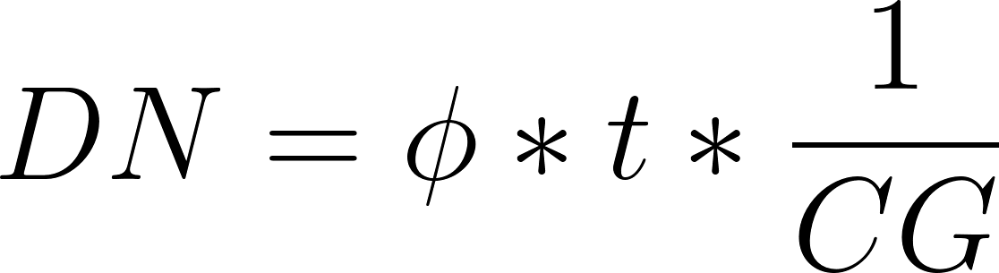
However, this equation does not account for saturation, so the maximum possible DN value must be calculated which will depend on the well capacity.

If the calculated DN value if greater than DNMax, the value will have to reset to DNMax.
Aptina CMOS Calculation
WC = 4192 e
CG = 1.8 e/dn


SNR Methods
We will consider 3 different methods of dealing with noise in our image.
Method 1
No noise, just calculate expected dn value per pixel.
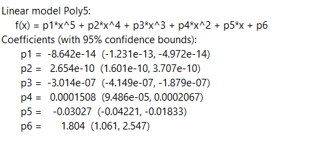
Method 2 (Specific to Aptina CMOS)
These values were experimentally determined and converted to equations using curve fitting. All of these noises are calculated in standard deviation. Furthermore, the noise is in units of DN.


Add noise in quadrature for total noise:

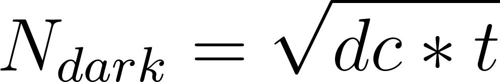
Method 3: General Noise Equation
Calculate in electrons then use conversion gain to convert to dn.
e: electrons
dc: dark current (e/s)


We can convert to DN by dividing the total by the conversion gain. We can substitute e = CG*dn so we can directly compare methods 2 and 3.
Noise Comparison
From Aptina CMOS Specifications:
dc = .88 e/s
nr = 4.42 e
We can also express electrons in DN so we can compare it to our previous method.
We will assume t=0 as the dark current is not statistically significant.
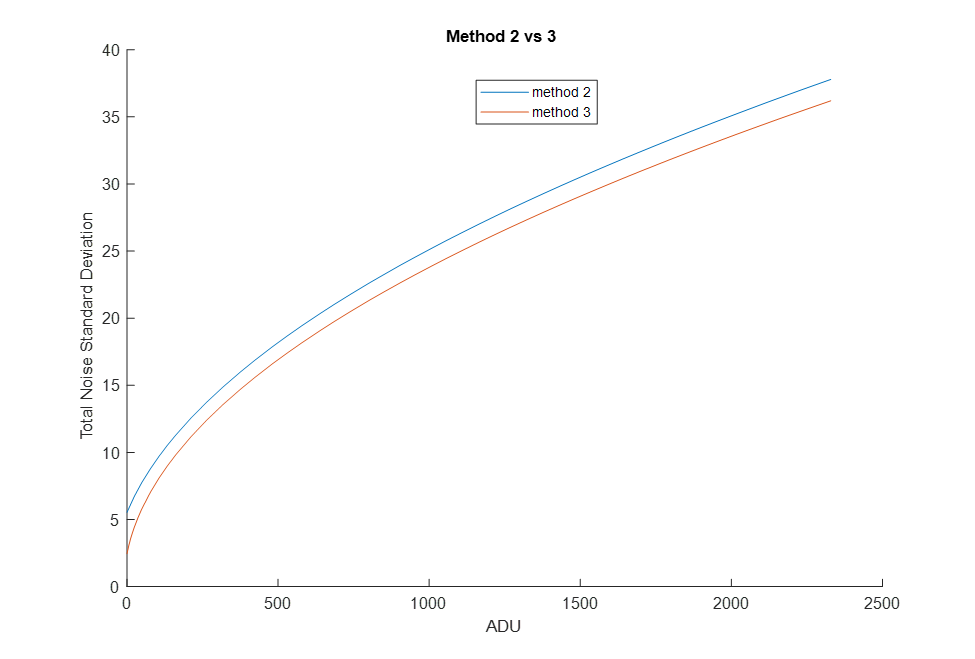
The biggest difference between the two methods is for pixels close to 0.
Applying Noise
In order to apply the noise, we need a gaussian random number generator that takes input mean (dn value) and the calculated standard deviation. We will use the Python module ‘random’ to do this.
One issue with this method is the dn value could go below 0 or above 2329. The difference is very important at 0 since proportional to the dn value, the noise has a much greater effect. Therefore, we will add the absolute value of the minimum value to every pixel. Then, we would reset any value above 2329 back to 2329 since this would not have a major impact compared to dn values near 0.
