Who we are
Owen Isley, Undergraduate Class of 2020
Gabriel Ramirez, Graduate Class of 2020
Jackson Ding, Graduate Class of 2020
Justin Clifford, Undergraduate Class of 2020
Goergen Institute Data Scientists
Our advisors
Bernie Gigas, PE, Fellow Engineer, R & D lead at SPX Flow Inc.
Professor Ajay Anand, PhD, Deputy Director of the Goergen Data Science Institute
Description
Our project’s goal is to verify or reject the Caldwell-Fay (2002) equation which models the natural outflow of Lake Ontario using previously non-digitized data from the 1800s. The IJC uses this equation to regulate the lake’s outflows on a daily basis. Then, we use the updated equation to assess whether or not the Moses-Saunders Dam has significantly altered water levels in Lake Ontario from their naturally-occurring levels.
History
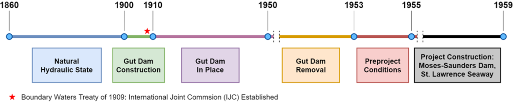
1. Natural Hydraulic State [1860-1900]
2. Gut Dam In Place [1910-1950]
3. Preproject Conditions [1953-1955)
The International Joint Commission (IJC) declares that the Lake Ontario outflow during the Preproject Conditions are to be used in the regulations Lake Ontario outflow after construction of the Moses-Saunders Dam and the St. Lawrence Seaway.
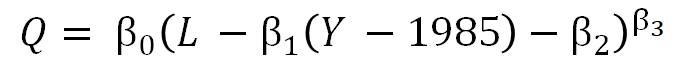
General Caldwell-Fay Equation (CFE)*

Q, Lake Ontario Outflow (m3 / s)
L, Lake Ontario Water Level (m)
Y, Year (continuous)
Calculates the natural hydraulic state Lake Ontario outflow (i.e., if the Moses-Saunders Hydro-power Plant and Seaway didn’t exist)
For the 2002 Caldwell-Fay Equation (CFE)+
β_0=555.823, β_1=1.5
* Excludes December, January, February, and March.
+ Lake Ontario Preproject Outlet Hydraulic Relationship; Caldwell, Fay (2002)
Project Goals
1. Do the Preproject Conditions accurately capture the Natural Hydraulic State?
2. Does the Caldwell-Fay Equation accurately predict the Natural Hydraulic State Lake Ontario outflows?
In Practical Terms: Does the Caldwell-Fay equation fairly represent the terms of the 1909 Boundary Waters Treaty?
Stitching Images
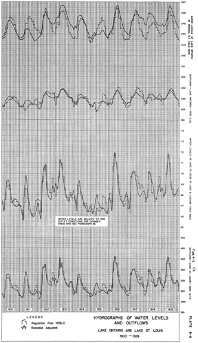
We were presented with newfound Lake Ontario data that went back to the year 1860, which meant we had the opportunity to work with data that had never been analyzed digitally before. However the data were a collection of disconnected line plots that are obviously non-digital given their age, and non-tabular as well as non-numeric.
But, if we could digitize these plots we would create the only existing digital dateset of measurements before any dam construction (“Natural Hydraulic State”). Since Caldwell and Fay’s original ambition was to model the lake’s natural behavior, we could use the actual “natural” data to verify the accuracy of the CFE, which can ultimately result in more accurate lake regulation going forward.
So, the backbone of our project was using this newfound (old) data to capture the behavior of the lake prior to any dam construction. We were able to secure high resolution PDFs scans of the graphs for us to work with, so the first challenge we faced towards actually digitizing was stitching the individual PDF pages together to re-construct continuous graphs. The plots represent the lake’s outflows and water level over time.
Curve Tracing
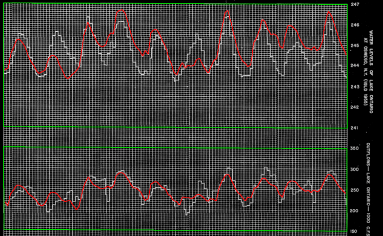
•Green lines calibrate pixel locations to real values.
•Algorithm then used to extract raw data form images.
•Convert water level from 1955 to 1985 International Great Lakes Datum
After stitching together the plots, we traced the water level and outflow graphs meticulously by hand to capture the form of the plots. We then used a feature in GIMP to capture the scale of the axis so that thousands of (x,y) values can be synthesized from our traces automatically. By doing so we constructed a data set of points that exactly model the plots, thereby reverse engineering a digital representation of the provided data.
For whatever reason the reference point from where the water level measurements were taken was changed in 1985, so a conversion was necessary to account for this (1985 Great Lakes Datum).
Correlation of CFE with Digitized Data
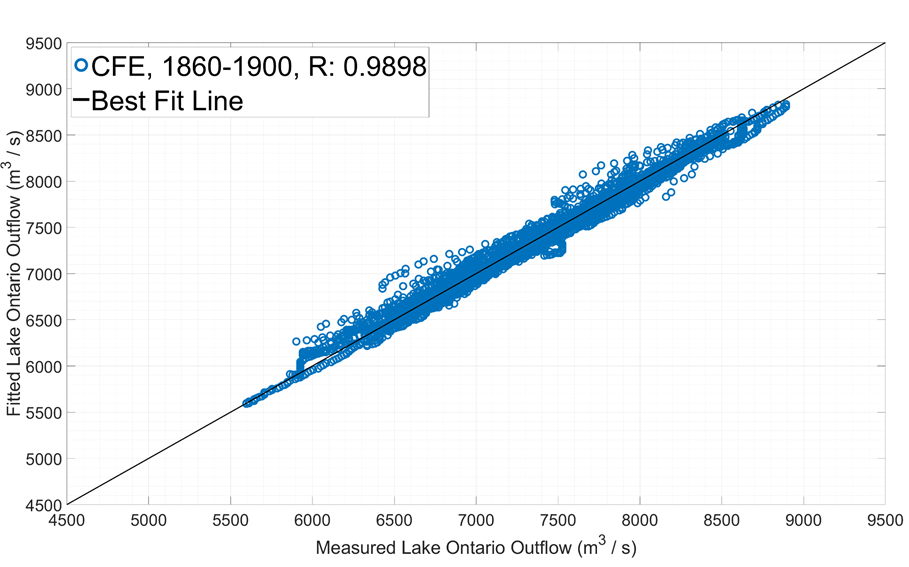
| Year | R |
| 1860-1900 | 0.9898 |
| 1910-1950 | 0.9961 |
| 1953-1955 | 0.9950 |
| 1860-1955 | 0.9940 |
Correlation of Regression with Digitized Data
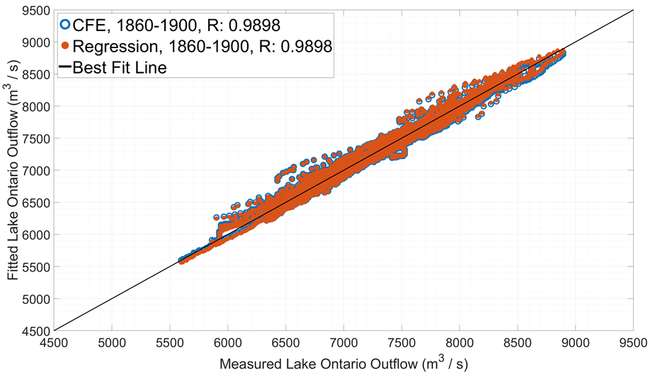
| Year | R |
| 1860-1900 | 0.9898 |
| 1910-1950 | 0.9961 |
| 1953-1955 | 0.9950 |
| 1860-1955 | 0.9939 |
Regression Coefficient Confidence Intervals
| 1860-1900 | Lower 99CI | Upper 99CI | Coefficient | CFE |
| β0 | 526.186 | 526.430 | 526.308 | 555.823 |
| β1 | 1.524 | 1.540 | 1.532 | 1.5 |
| 1910-1950 | Lower 99CI | Upper 99CI | Coefficient | CFE |
| β0 | 528.078 | 528.222 | 528.150 | 555.823 |
| β1 | 1.525 | 1.535 | 1.530 | 1.5 |
| 1953-1955 | Lower 99CI | Upper 99CI | Coefficient | CFE |
| β0 | 608.767 | 612.373 | 610.570 | 555.823 |
| β1 | 1.422 | 1.470 | 1.446 | 1.5 |
| 1860-1955 | Lower 99CI | Upper 99CI | Coefficient | CFE |
| β0 | 527.752 | 527.840 | 527.796 | 555.823 |
| β1 | 1.526 | 1.534 | 1.530 | 1.5 |
“1860-1900”, “1910-1950”, and “1860-1955” were very similar. “1953-1955” no similarity. “CFE” no similarity.
Bootstrap Fitting*
* Excludes December, January, February, and March.
Where:
Q, Lake Ontario Outflow (m3 / s)
L, Lake Ontario Water Level (m)
Y, Year (continuous)
Bootstrap Algorithm:
•Global search algorithm
•Randomized initial parameters
•Bootstrap samples: 1000
•Randomized sample size: 195
Model Summary
| Model Name | Fitting Method | Time Interval | β_0 | β_1 | β_2 | β_3 |
| CFE | Regression | 1953-1955 | 555.823 | 0.0014 | 69.474 | 1.5 |
| A | Regression | 1860-1900 | 526.308 | 0.0014 | 69.474 | 1.5 |
| B | Regression | 1910-1950 | 528.150 | 0.0014 | 69.474 | 1.5 |
| C | Regression | 1953-1955 | 610.570 | 0.0014 | 69.474 | 1.5 |
| D | Regression | 1860-1955 | 527.796 | 0.0014 | 69.474 | 1.5 |
| Boot A | Bootstrap | 1860-1900 | 560.284 | 0.0018 | 69.574 | 1.506 |
| Boot B | Bootstrap | 1910-1950 | 568.594 | 0.0019 | 69.587 | 1.502 |
| Boot C | Bootstrap | 1953-1955 | 588.960 | 0.0015 | 69.423 | 1.459 |
| Boot D | Bootstrap | 1860-1955 | 569.789 | 0.0015 | 69.571 | 1.501 |
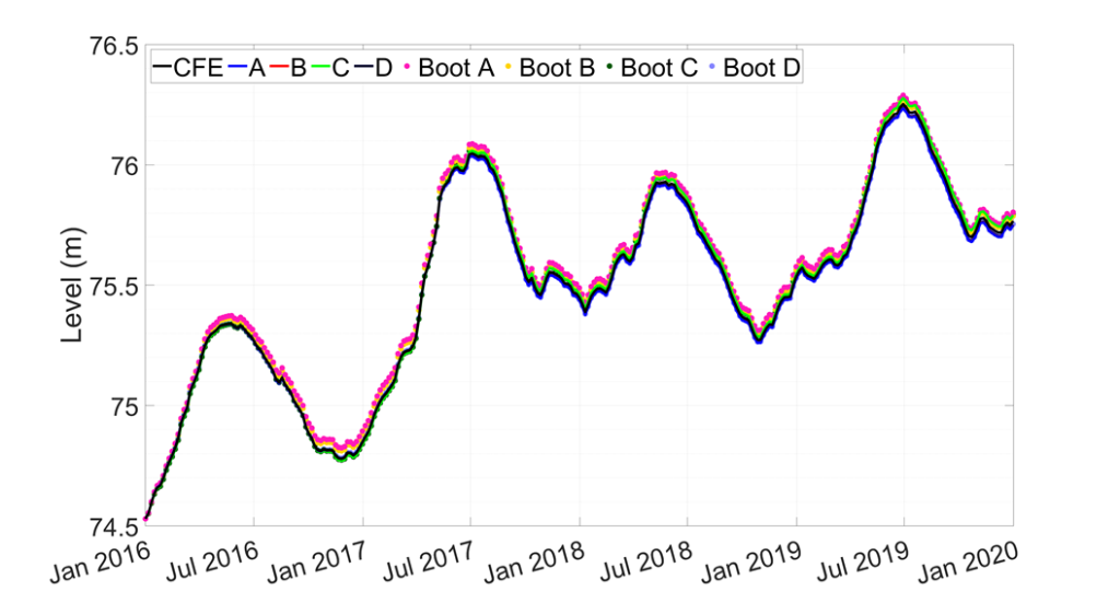
Predicted Water Level
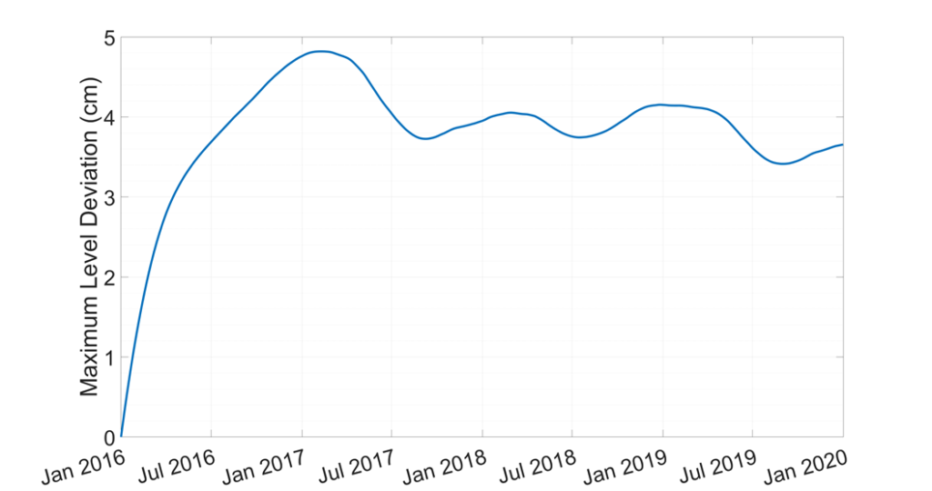
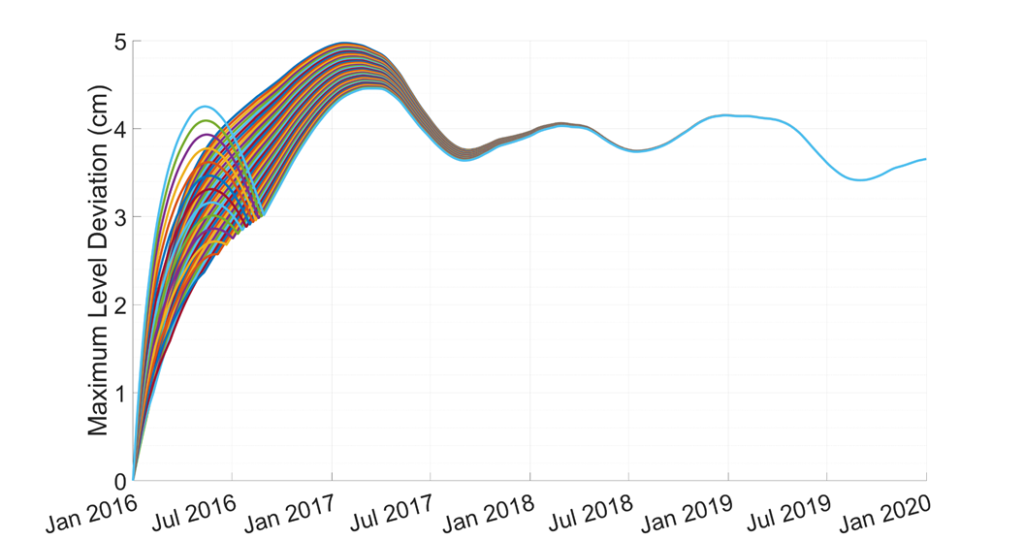
Maximum Water Level Deviation
Limited Sensitivity Analysis
Conclusion
Overall, we conclude that the predictive equation estimated by Caldwell and Fay holds true for all practical purposes; the correlation between measured values and fitted values predicted by the Caldwell-Fay Equation is nearly perfect for all three time periods, as well as the pooled sample of these three time periods. Further, the models we estimate ourselves match nearly perfectly with what Caldwell-Fay would have predicted, regardless of the time period in question. And although some estimated coefficients tend to differ significantly from Caldwell-Fay from a statistical standpoint (specifically, β0 tends to be distinct from what Caldwell and Fay estimated) the physical differences are negligible; our Maximum Water Level Deviation and Limited Sensitivity Analysis components show that in the worst case, none of our predictions of natural water level would have underestimated true water levels by more than 5 cm at any point over the last 4+ years. The practical takeaway of this project is that the Moses-Saunders Dam has not significantly altered water levels in Lake Ontario away from their naturally-occurring levels, and thus the construction of this dam has not violated the Boundary Waters Treaty.