1. Introduction
Investment, based on the definition of Robinhood (one famous online brokerage platform), is the attempt to buy assets (stocks, real estate, etc.) with own resources (money or credit) for the sake of future profits [1]. In the stock market, investors typically trade stocks in two different ways to gain future profits: a long position and a short position. As explained by the Office of Investor Education and Advocacy from the U.S. Securities and Exchange Commission [2], having a long position means owning a security, while having a short position means selling a security that the investor does not yet own. In a long position, investors buy and own securities in the belief that they can sell the securities at higher prices in the future to gain profits. In a short position, the investors sell securities they do not yet own at current prices and will later buy securities at new prices to fulfill their sales, in the hope that the securities’ prices will decrease over time.
One straightforward trading strategy based on the two positions is momentum trading. Bhardwaj et al. defined the strategy as buying securities that have exhibited strong recent performance and selling securities that have exhibited weak recent performance in their 2015 publication Momentum Strategies in Futures Markets and Trend-Following Funds [3]. Their idea is that the securities that have performed well or poorly in the past exhibit momentum and are likely to continue performing well or poorly in the future. They also discussed one major risk of momentum trading strategies: there may be large losses when there are large drawdowns during periods of market volatility.
Considering the high risk of investing in single stocks, Elton et al. explained how the risk of single-stock investment can be diversified through investing in portfolios (multiple stocks together) in their book Modern Portfolio Theory and Investment Analysis [4]. However, the risk of momentum trading still persists. Without regarding the difficulties of accurately predicting stock prices, the increasing trend seems to be easier to capture in a bull market (a market that is on the rise and where the conditions of the economy are generally favorable). While the decreasing trend is easier to capture in a bear market (the market in an economy that is receding and where most stocks are declining in value), short positions are usually harder to achieve considering the availability of shares that can be borrowed.
Considering the availability of the two positions and the market risk, pairs trading takes a different approach compared to momentum trading which aims to avoid market risk and is therefore market neutral. As described in The Definite Guide to Pairs Trading [5], the pairs trading strategy takes advantage of the mispricing of two co-moving assets and buys a long position in the undervalued asset and a short position in the overvalued asset. To be specific, a pair of co-moving assets are likely to have a price difference between stationary around a certain value in the long term. When such a price difference (spread) of the pair significantly deviates from its long-term mean, it is very likely that either one asset is overvalued, another asset is undervalued, or both, and therefore the spread of the pair is very likely to revert to its long-term mean (mean-reverting). The difference between a pairs trading strategy and other strategies that involve long-short equity is that pairs trading strategies trade strictly on pairs of stocks: it will always take a long position on one stock and a short position on the other; long-short equity, on the other hand, does not require such a one-on-one match.
Our sponsor FLX AI, who “offer scalable solutions that deploy artificial intelligence and big data to the cloud” [6], hopes to utilize the big data in the stock market and wants us to develop a pair strategy from data science approaches that can outperform S&P 500, a stock market index that measures the performance of 500 large-cap U.S. companies listed on the New York Stock Exchange (NYSE) or the NASDAQ stock exchange. We will develop a pairs trading strategy that selects stocks from the list of S&P 500 stocks, and we will compare the final performance of our strategy with SPY, an exchange-traded fund that tracks the performance of the S&P 500 [7].
2. Data Set Description and Exploratory Analysis
Since the project aims at making profits with pairs trading, the dataset is simply the past prices of the stocks in S&P 500. Unlike common datasets, it is not a simple CSV or Excel file. Instead, the QuantConnect online platform records all the price data and offers its users various functions to retrieve and manipulate it. Figure 1 is an example of how QuantConnect provides the price data to the users.
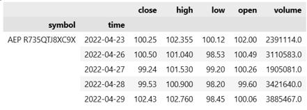
Figure 1. A Visual Example of the Price Data
The symbol column is the symbol for each stock and the volume column represents the total amounts of trades made on this day. The open and close columns are the daily opening and closing prices, while the other two are the highest and lowest prices on this day. For our later analysis, we will use the closing prices as the training data, to conduct pair selection and build spread models. After the training process is done, we will use the hourly stock price to test the performances of our algorithms. This is because hourly data is more flexible and fluctuating and it will be easier for us to detect and manipulate the bugs existing in our methods.
3. Model Development
According to The Definitive Guide to Pairs Trading [5], there are 3 main steps to building a pairs trading algorithm: pair selection, spread modeling, and trading rules development. Pair selection aims to find co-moving assets with similar returns and mean-reverting spread. Spread modeling aims to simulate the spreads of the selected pairs in a way that can maximize profits and ensure market neutrality. Trading rules development aims to set additional rules (other than entry and liquidation rules) to control short-term loss.
3.1 Pair Selection
To perform pairs trading, an essential element of the algorithm is to identify co-moving pairs. Without high-quality pairs, the algorithm would not be effective and profitable no matter how complicated and advanced the spread modeling and trading rules are. The pair selection pipeline could be decomposed into three parts: data preprocessing, clustering, and testing against selection rules [5].
3.1.1 Data Preprocessing
Recall from the introduction, an important feature of good pairs is having similar returns. While the dataset from QuantConnect does not directly contain the information, we constructed the daily return feature by ourselves. For each individual stock, we calculated the percentage of price changes between two consecutive days using only the closing price and dropped data for the earliest date in the dataset since the return values could not be calculated for the first day. We then pivoted the dataset so that it was indexed by stock symbols and had each column recording the daily return percentage. Figure 2 provides a visual representation of the steps above.
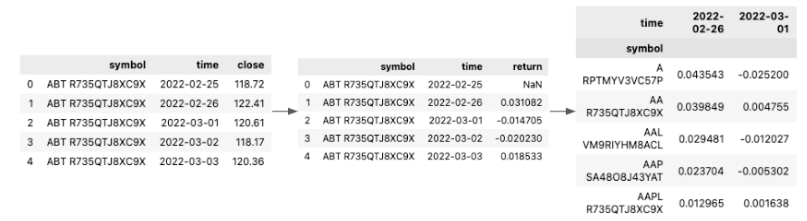
Figure 2. A Visual Representation of the Data Preprocessing Steps
We then performed scaling and dimensionality reduction on the daily return data since having one column for an additional day in the dataset would be unnecessary and computationally burdensome. We found that, while keeping other algorithm parameters unchanged, a higher threshold on the explained variance resulted in more selected pairs finally, and thus decided to keep whatever number of features needed to reach a 0.8 explained variance level.
3.1.2 Clustering
Clustering is a crucial step in the pair selection pipeline because it helps to identify stocks with similar returns. Without clustering, a candidate pair could be formed using any two stocks in the trading scope. On the other hand, with clustering, only the stocks with similar returns (i.e. in the same cluster) could form a candidate pair, which helps to significantly reduce the size of search space for the final eligible pairs. In our project, we conducted OPTICS clustering on the preprocessed dataset and set the min_samples parameter to 3. We had a preference for a smaller value of min_samples since it would yield more and smaller clusters, which means a smaller search space than having a large min_samples value with fewer but larger clusters.
3.1.3 Selection Rules
After clustering, each stock in a particular cluster is paired up with each other stocks left in the same cluster to form a candidate pair. For example, a cluster with n pairs will yield
n2=n!2! (n-2)!! pairs
Having similar returns only satisfies one of the two requirements for being qualified pairs. While having stationary and mean-reverting spread is the other requirement, each candidate pair needed to pass 4 additional selection rules to be considered as an eligible pair [5]:
- Cointegration test: A statistical test determining whether there exists a that makes the spread of the two stocks stationery. We set a lenient p-value threshold at 0.1 for more potential pairs. The spread of two stocks is defined as follows:
spread = priceA – β × priceB
- Hurst exponent: We calculated the Hurst exponent of the spread series using the hurst python library. A smaller Hurst exponent closer to 0 means that the series has a stronger tendency to return to its long-term means [8]. Since we desired the spread to be mean-reverting, only pairs with a Hurst exponent less than 0.5 could pass the test.
- Mean reversion half-life: We also measured how long it takes for the spread to revert to its mean [9]. A short half-life means quick reversion and may indicate instability, while a large half-time means slower reversion and indicate fewer trading opportunities. Therefore, pairs with half-time either shorter than 1 day or longer than 1 year would fail this test.
- Number of annual mean crosses: It is another measurement of the frequency of mean reversion. For qualified pairs, the spread needs to cross its means more than 12 times a year to provide sufficient exiting and liquation opportunities.
3.1.4 Sample Results and Attempt of Improvement
To test the effectiveness of our pair selection methods, we ran the algorithm using 10 months of data ranging from March 2022 to December 2022. The algorithm generated 258 candidate pairs while 2 of them were identified as qualified pairs as listed in Table 1.
Table 1. List of pairs picked by the pair selection algorithm.
|
Pairs |
Company A |
Industry A |
Company B |
Industry B |
|
Pair 1 |
Zions Bancorporation |
Financial Service |
Comerica Incorporated |
Financial Service |
|
Pair 2 |
Kinder Morgan Inc |
Energy |
Williams Companies, Inc. |
Energy |
We noticed that both of the stocks in the two pairs belong to the same industry. This aligns with what we summarized from our literature review, which says that constituents of a pair tend to come from the same industry sector [10]. However, at the same time, we noticed that our algorithm was yielding very few pairs, which is undesirable since it indicates fewer trading opportunities and potentially a lower return. To improve the algorithm, we tried to add more features to the original dataset by retrieving the price-earnings data (PE ratio). We performed similar data preprocessing steps and reran the algorithm. The algorithm generated 15 pairs, which was indeed an improvement over the original amount. The following Table 2 provides some examples of the selected pairs.
Table 2. Examples of pairs picked by the UPDATED pair selection algorithm.
|
Pairs |
Company A |
Industry A |
Company B |
Industry B |
|
Pair 1 |
The Allstate Corporation |
Insurance |
Johnson and Johnson |
Healthcare |
|
Pair 2 |
Kellogg Company |
Food |
NVIDIA Corporation |
Manufacturing |
However, with the added feature, we noticed that now the constituents of the same pair do not belong to the same industry anymore. After trading the two sets of pairs, both from the original model and the updated model, using the same trading logic, we find that the original pairs yielded a significantly higher return (6.52%) than the update pairs (-1.15%) on a backtest ranging from January 2023 to March 2023. Therefore, we concluded that, although adding the PE ratio data increased the number of pairs selected, it decreased the quality of pairs, and thus we decided to use our original algorithm in our final code.
3.2 Spread Modeling
After identifying the co-moving pairs, the second step would be modeling the spread of two stocks within each pair. In this project, we found two aspects of stock data to simulate and model the spread: either by direct inferencing from the historical prices or from the historical returns of the pair. We developed the Bollinger Band approach and OU Probabilistic Forecasting approach based on the historical prices; we developed the Copula approach and Cointegration approach based on the historical returns.
3.2.1 Bollinger Band
Since we know that the selected pairs from the previous step will have stationary and mean-reverting spreads, a trading opportunity appears when the spread of the pair deviates too far away from its mean. This is because we could ultimately expect the spread to return to the mean. To quantify this idea, we set the 20-day moving average of the spread to be the baseline and defined “deviates too far away” as being either higher than 2 times the 20-day rolling standard deviation above the baseline or lower than 2 times the 20-day rolling standard deviation below the baseline. The acceptable deviation from the mean is represented by the grey area below in Figure 3, and once the spread leaves the grey area, we regard it as a trading opportunity and would start a position.
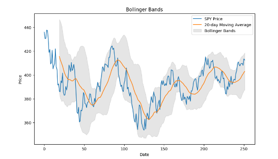
Figure 3. A Visual Representation of the Bollinger Band
Recall that the spread is the linear transformation of the price difference between stock A and stock B. When the spread goes above the Bollinger band, either stock A is overpriced or stock B is underpriced, and we will therefore short stock A and long stock B. When the spread goes below the Bollinger band, using similar logic, we will long stock A and short stock B instead. The proportion of capital used to trade stock A and stock B will be calculated in the next step (please refer to section 3.2.2). Under the Bollinger band idea, we would exit the position when the spread returns and touches its mean again.
3.2.2 Probabilistic Forecasting based on Ornstein–Uhlenbeck Process
While the selected pairs are all qualified under the mean-reverting constraint, which makes spread forecasting based on moving averages a feasible approach, we want to gain a better understanding of the daily changes in the spread of pairs, and a feasible way would be representing the spread using Ornstein–Uhlenbeck process (OU process) [11]. The OU process is defined by the stochastic differential equation:
dxt=( –xt )dt+dWt
In the setting of pairs trading, if we let xt be the portfolio value (spread) of pair x at time t, then would be the mean reversion speed, would be the long-term mean of the portfolio value, would be the instantaneous volatility, and Wt would be the Wiener process [X]. With the equation, our goal is therefore to find out the set of parameters that can best explain and represent the actual change of portfolio value. We can achieve this maximum likelihood estimation (MLE) with the following log-likelihood function [X]:
L(,,|Xt)=-12ln(2)-ln()-12n2i=1n[xi–xi-1e–t–(1-e–t)]2
However, we also have to know the proper weight, and , of each stock, S1and S2, in pair x to calculate the xt:
xt=St1–St2
Since the sum of stock weights and should always be 1 within pair x, all we need to do is finding out an optimal that maximize the log-likelihood function and we will automatical find out the optimal .
In actual implementation, we achieved the MLE of OU process equation by finding out the corresponding set of , , and that minimize the negative log-likelihood function (which is equivalent to maximizing log-likelihood function) for each of the possible stock weight ranging from 0.01, 0.02, to 1.00. We would select the set of and OU process equation parameters that have the largest log-likelihood.
With the set of optimal weights and parameters, we can use the differential equations of OU process to forecast the future portfolio value of pair x (time t) based on the portfolio value from the previous day (time t-1):
xt=xt-1+dxt
In our actual implementation, we modified the forecasting equation as [12]:
xt=xt-1+( –xt )t+t N(0,1)
Since our implementation include a random process based on Normal distribution, each individual forecast on the same time t would have different values. Therefore, we took the probabilistic forecasting approach. For each time t, we would make 20,000 forecasts, and we would use the mean of the 10,000 forecasts and the 98% confidence interval as the probabilistic forecast. A sample OU probabilistic forecasting of the portfolio value of the pair American Electric Power Company and WEC Energy Group (selected by our pair selection method) with a 5-day forecasting window, as shown in Figure 4, could show how the actual portfolio value would generally stay within the confidence interval of forecasts.
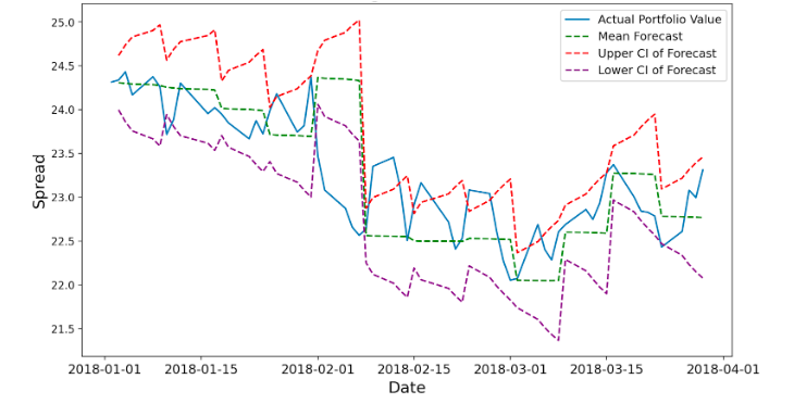
Figure 4. Example Probabilistic Forecasting with 95% Confidence Interval
Nevertheless, since we are forecasting based on another forecast for any forecasting window larger than 1 day, our forecasting error will sum up every day. In Figure XX, the summation of error can be seen by the increasing range of the confidence interval each day within each forecasting window. To control the forecasting error, we limited the length of the forecasting window. Specifically, we used a forecasting window of 10 days when the return based on the pairs trading algorithm based on OU Probabilistic Forecasting approach is positive and used a forecasting window of 5 days when the return is negative.
To use the forecasted spread based on the OU process in pairs trading strategy, we incorporated the OU probabilistic forecasting into the Bollinger Bind approach: we replaced the moving average of portfolio value with the mean of probabilistic forecast and replaced the range of 2 standard deviations upper and lower the moving average by the 98% confidence interval of the probabilistic forecast. The entry and liquidation logic, therefore, remained the same as the Bollinger Band approach.
3.2.3 Copula
While the other methods look at the daily closing prices and build their trading logistics, the Copula method instead trains the daily returns and determines how to trade with the percentiles of the daily returns. The basic idea is that on every trading day, we get quantile functions of the return series for each stock in the selected pair of the past year, and turn the return data into percentiles, which represent the rankings of the return on this day in the past year.
With the percentiles, we are able to set up the copula function and derive our trading signals. Besides the two quantiles of the two stocks in the pair, we need another fixed coefficient θ, which can be calculated from the Kendall’s correlation coefficient of the returns. In our project, we mainly select three categories of Copula and Figure 5 below is the calculations of θ for these three methods given by QuantConnect [13].
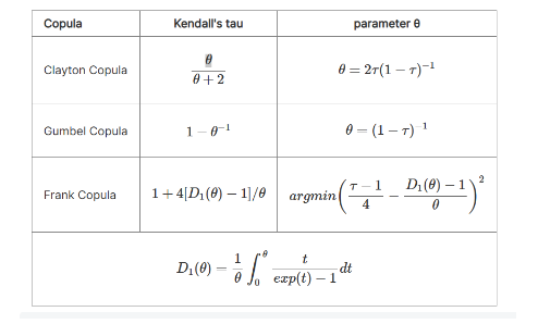
Figure 5. θ Calculations in Copula Algorithm
With the quantiles of the returns and the θ, we will be able to build up the Copula conditional probabilities. Since we have three categories, we absolutely have to build three pairs of conditional probabilities, and each of them is complete and can be used for real-world trades [13].
The Clayton Copula functions are:
C(u|v)=v–θ-1(u–θ+v–θ-1)–1θ-1
C(v|u)=u–θ-1(u–θ+v–θ-1)–1θ-1
in which u and v are the percentiles of the returns.
The Gumbel functions are:
A=ln(u)–θ+ln(v)–θ
C=exp(A–1θ)
C(u|v)=C[-ln(u)θ-ln(v)θ]1-θθ[-ln(v)]θ-11v
C(v|u)=C[-ln(u)θ-ln(v)θ]1-θθ[-ln(u)]θ-11u
The Frank functions are:
C(u|v)=(exp(−θu)−1)(exp(−θv)−1)+(exp(−θv)−1)(exp(−θu)−1)(exp(−θv)−1)+(exp(−θ)−1)
C(v|u)=(exp(−θu)−1)(exp(−θv)−1)+(exp(−θu)−1)(exp(−θu)−1)(exp(−θv)−1)+(exp(−θ)−1)
The Copula conditional probabilities represent the actual quantiles of the two stocks in the past year and therefore, by merging the idea of pairs trading, we can translate the signals into positions and generate the basic training rules:
Opening rules:
If C(u|v) ≦ blowAND C(v|u) ≧ bup, then stock 1 is undervalued, and stock 2 is overvalued. Hence we long the spread. (1 in position)
If C(v|u) ≦ blowAND C(u|v) ≧ bup, then stock 2 is undervalued, and stock 1 is overvalued. Hence we short the spread. (-1 in position)
Exit rule:
If BOTH/EITHER conditional probabilities cross the boundary of 0.5, then we exit the position, as we consider the position no longer valid. (0 in position) [5].
Basically, the idea is that we open a trade by longing the undervalued and shorting the overvalued. When the returns cross the mean sometime in the future, we end this trade by selling all the shares we own.
3.2.4 Cointegration
Cointegration is an essential concept in pairs trading due to its multiple usages. It can be implemented in all three stages: pair selection, spread modeling, and trading rules development. Formally, Cointegration is a statistical test technique that examines the relationship between two or more non-stationary time series over a prolonged period or a specified timeframe. It is used to establish long-term parameters or equilibrium between two or more variables. Additionally, it identifies situations where two or more stationary time series are cointegrated, indicating that they will not deviate significantly from equilibrium over an extended period. The cointegrated series(Zₜ) for two stocks particularly can be expressed as [5]:
Zₜ = (mt) – β(nt) = (vₘₜ – βvₙₜ) + (εₘₜ – εₙₜ),
where mt, nt are the two co-moving stocks, εₘₜ-εₙₜ is the residual difference.
The definition of cointegration informs that if one asset deviates from its long-term equilibrium, it will eventually revert back to it, pulling the other asset along with it. This behavior is also known as mean reversion. Therefore, we can utilize this property to make arbitrage during this process; we follow the fundamental principle of investing: “buy undervalued and sell overvalued” [5]. The assets in Figure 6 are one of our pairs that actually traded in our algorithm. We can see that these two assets have overall the same co-moving trend despite the price difference and thus being identified as cointegrated.
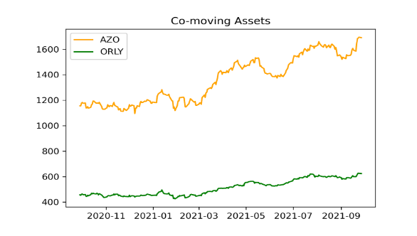
Figure 6. Cointegrated Assets
After getting the pairs from the pair selection algorithm, we utilize the two securities as the outcome and independent variable for the OLS(Ordinary Least Square) regression model and get the parameter β by fitting the regression model. The next step is to check the cointegration of every moving window. At this time, we included in KPSS(Kwiatkowski–Phillips–Schmidt–Shin) test. It not only checked the stationarity around a deterministic trend but also help us to optimize our β to maximize the stationarity by utilizing optimization methods such as the Nelder-Mead algorithm.
The trading logistic for cointegration is similar to most of the other strategies but one difference. We set up a significance level of 5% for our maximum KPSS score, which is 0.463, and we only trade if the current KPSS score is smaller than this threshold, otherwise, we liquidate the assets.
4. Trading Rules Development
With our spread modeling methods and the identified entry and exit point, we developed three additional trading rules to maximize our returns.
4.1 Pairs Update
During our project, we found that good pairs were not persistent. For example, a qualified pair in 2018 may not still be qualified in 2023 as shown in Figure 7. Therefore, it is essential for our trading algorithm to keep the selected pairs updated, and in our algorithm design, we set two triggers for the pair selection to rerun and refresh its results.
- Condition 1: When the last pair selection was performed more than 6 months ago. The pair selection will be refreshed to provide a new set of pairs to trade on.
- Condition 2: When the overall expected return (the return that would be achieved if exits the position today at the current price) of the entire portfolio is lower than a pre-defined threshold (e.g. -10%), it may indicate that there might be low-quality pairs in the pair selection results from the last refresh. Then, the pair selection algorithm would be triggered no matter when the last refresh was.
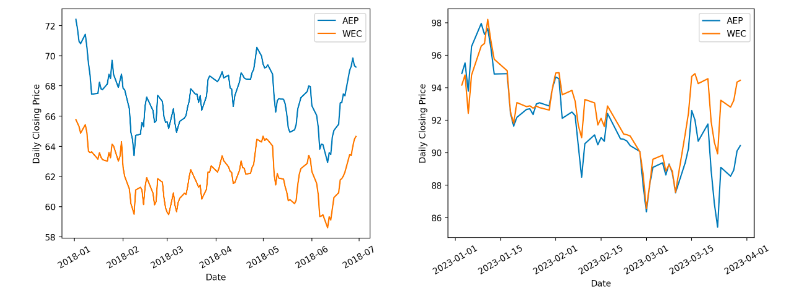
Figure 7. An Example Proving that Pairs Could Be Outdated
4.2 Loss Control
Thinking from the investor’s perspective, there is always a limited acceptance of the loss of the investment. Therefore, in our case, we set the algorithm to exit the position of a pair when the expected return of the particular pair falls below a certain pre-defined threshold (e.g. -5% or -10%). Although triggering such a mechanism books a loss on the portfolio, it prevents us from keeping betting on a pair that is already proven risky and eliminates the possibility of generating more future losses.
4.3 Prediction Update
The last rule that we considered was more specific to the OU process approach. When the prediction deviates from reality (as shown in Figure 8), it would also cause the algorithm to yield low daily returns. As a result, when we observed that the daily return (instead of the expected return) of a pair is lower than a pre-defined threshold, it might indicate that the forecast from our OU approach was inaccurate, and thus, in this case, we would set the program to rerun the forecasting process again using the lasted data to improve the accuracy.
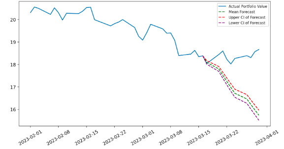
Figure 8. Forecast Deviation Using 95% Confidence Interval
- Results
The table (Table 3) below shows our strategies’ performance during 2022 using backtesting. It shows that SP&500 did a really terrible job in 2022, it yielded an overall return of -18.11% with a maximum drawdown of -25.70%. Clearly, all of our strategies beat the market and we all generated positive returns. Specifically, the OU-process-based algorithm yielded a return of 11.53% exclusively with an acceptable maximum drawdown. Copula also has a return of 8.13% with a low maximum drawdown of 1.40%, which is also a strategy that we satisfy.
|
OU |
Bollinger |
Copula |
Cointegration |
SPY |
|
|
Return |
11.53% |
3.66% |
8.13% |
3.76% |
-18.11% |
|
Annual Variance |
0.022 |
0.002 |
0.001 |
0 |
0.04 |
|
Max Drawdown |
-12.50% |
-3.00% |
-1.40% |
-1.10% |
-25.70% |
|
Number of Trade |
1615 |
164 |
208 |
106 |
1 |
Table 3. 2022 Performance
The table (Table 4) recorded the overall performance of our strategies during 2021. In contrast, SP&500 attained a return of 28.78%, which is superior. The only algorithm that can compete with SP&500 is still the OU algorithm, with a return of 28.10%. While other strategies all yielded positive returns, our goal is to outperform the market index. Therefore, we selected the OU algorithm as our final strategy.
|
OU |
Bollinger |
Copula |
Cointegration |
SPY |
|
|
Return |
28.10% |
10.51% |
3.38% |
19.45% |
28.78% |
|
Annual Variance |
0.022 |
0.003 |
0.019 |
0.003 |
0.012 |
|
Max Drawdown |
-11% |
-3.60% |
-18% |
-3.40% |
-5.50% |
|
Number of Trade |
528 |
92 |
44 |
6 |
1 |
Table 4. 2021 Performance
We also found that the performance of pairs trading algorithms is actually correlated with the market trend. 2022 is a bear market, where investment prices drop dramatically, while 2021 is a bull market, where investment prices increase steadily. We infer that during a bear market, there are more fluctuations and statistical arbitrage opportunities. Therefore, pairs trading is more fit for the bear market.
- Conclusion & Future Work
As clarified formerly in this report, we have built up our own pairs trading strategy, and after careful online backtesting, we have achieved the highest return of 11.53% in 2021 in comparison with the -18.11% return of SPY in the same year, using the probabilistic forecasting based on the OU process.
Initially, with OPTICS clustering, we generate the candidate pool and conduct our four selection rules, therefore deriving the final optimal co-moving pairs that will be manipulated in our trades. Subsequently, we involve four distinct spread modeling methods including Bollinger Band, OU process, Copula, and Cointegration, whose basic idea is simple–open a trade when extreme price or return appears, and close the position when it returns back to its mean.
Afterward, we also added the pair update logic and the loss control logic to our algorithm because pairs are evolving as time goes and we may sometimes suffer from great losses. Besides, for the OU process, the specific prediction update logic is added to the OU process because it is a probabilistic forecasting process, and sometimes bad predictions occur.
For the future steps, there are some aspects for us to consider. We have noticed that our results are very sensitive to the time span of the training data. When we change the time span in the pair selection or spread modeling, our return value can change at a very large scale and very fast speed. It even experienced a 20% change when the time span increased by one month. Therefore, a significant step is to try more testing and look for ways to stabilize this change.
Besides, in our testing phase, we were using the hourly resolution, which means the data is recorded every hour. We would like to try different time resolutions such as daily resolutions to see if the results will differ, as stock prices may be frequently fluctuating when actively traded.
Reference
[6] “About FLX AI – FLX AI.” https://flxai.com/about-flx-ai/ (accessed Apr. 30, 2023).