Who we are
Haoyu Chen, Undergraduate Class of 2021
Xinyu Hu, Undergraduate Class of 2021
Yiwen Cai, Undergraduate Class of 2021
Yuchao Zhao, Undergraduate Class of 2021
Our Advisors
Professor Ajay Anand
Professor Pedro Fernandez
Customer
Paychex, Inc.
1. INTRODUCTION
Nowadays, business is not just simply selling a product to customers; instead, firms are looking for the “right” potential clients and sell them the “right” products, which, based on this concept, can significantly improve the efficiency of a business. Consequently, knowing the information of their customers becomes a fundamental issue for companies. More importantly, the reason that a client purchases their product is another critical point. As a result, the concept of “User Persona” was invented, which became an indispensable business and marketing analysis factor. According to Airfocus’s article, “What Is a User Persona?” a user persona is a semi-fictional character created to represent different customer types that use a company’s products or services [1]. The user persona can reflect the common attributes across a group of people, which means we can use a specific pattern to describe a particular group of people because they share lots of characteristics. This analysis method intends to give a reliable and realistic reflection of how a business could expect a group of people to engage with a product, service, or campaign [1].
Paychex is a leading company in the HR software industry. Its solutions cross a wide range of businesses, including Payroll Service, Employee Benefits, HR Services, Time&Attendance, and Business Insurance. Paychex can help the owners and HR managers of small to medium-sized businesses manage employee records, streamline talent management, and access critical data to help them make informed business decisions with confidence [2]. In 2019, Paychex achieved a 12% increase in the total revenue growth and made $3.8 Billion in revenue for that fiscal year [3]. Thus, it is reasonable and practical for such an industry giant to do an in-depth analysis of their existing and potential customers. In turn, the company can be better focused on the right customers, reducing the time and resource that wastes on the impossible customers, and improve their products based on the scientific report and clients’ preference.
In this project, with the Paychex team, our group aims to help Paychex improve their sales of 401(k) service products to existing clients. Therefore, we separate this project into two stages. In the first stage, we investigated the probability that an existing client will add 401(k) services over the next three months. In this part, our group implemented the “Random Forest” prediction model to understand the range of probabilities that would be acceptable for the Paychex team. Our group also tried oversampling and undersampling methods to tackle the imbalanced target distribution. In the second stage, we inquired deeply into why a particular client may be a good candidate or a poor candidate. In other words, in this part, we began to learn and depict the “User Persona” of 401(k) service product. We conducted model explainers using LIME and SHAP to interpret specific instances. Since SHAP is exhaustive and guarantees better consistency and accuracy than the LIME model, it is very time-consuming. On the other hand, the LIME model only provides local fidelity; therefore, it could not offer any insights globally, but the model is swift to run. To make up for the global interpretation that the LIME model couldn’t deliver, we analyzed the SHAP summary plot to give recommendations based on the impact of features on the probability of adding the 401(k).
2. DATA DESCRIPTION
2.1 Data Collection
We received the data from the Paychex team through email. It’s a one CSV file containing about two hundred thousand rows, where each row represents one client so that we have information about two hundred thousand clients.
2.2 Data Overview
Figure 1 shows that the dataset contains 36 columns, including a pseudo ID number ranging from 1 to 200,000. But this column is meaningless for model training because we are not interested in the relationship between ID number and desire to purchase 401(k) services. The second column, Target, is a Boolean variable where 0 indicates the client did not add 401(k) services within three months, and 1 indicates the client added the services. It is the dependent variable of this project, and the rest 34 columns are independent variables.
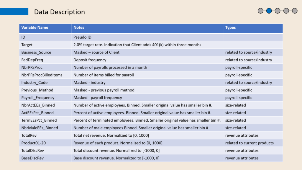
The dataset includes nine categorical features. For example, the fourth column indicates the deposit frequency classified into “monthly” or “semi-weekly.” On the other hand, product-related and revenue attributes are all numerical. The revenue features, TotalRev, TotalDiscRev, and BaseDiscRev, are normalized to [-1000,0]. Besides, there are also some columns with numerical data but transformed into categorical. For example, the “NbrActEEs_Binned” column represents the number of active employees. It should be numerical data originally, but it’s binned into groups, making it categorical.
2.3 Data Cleaning
2.3.1 Missing values: There is no missing value in any column.
2.3.2 Unusual values or Outliers: No noise or outliers.
2.3.3 Duplicates: There are no duplicated rows.
2.4 Data Preprocessing
First, we dropped the pseudo ID column because it has no real-world meaning. The second thing is to use one-hot-encoding to transform all the categorical data to Boolean variables to suit the machine learning models and explainers that we are going to apply.
3. EXPLORATORY ANALYSIS
3.1 Data Visualization
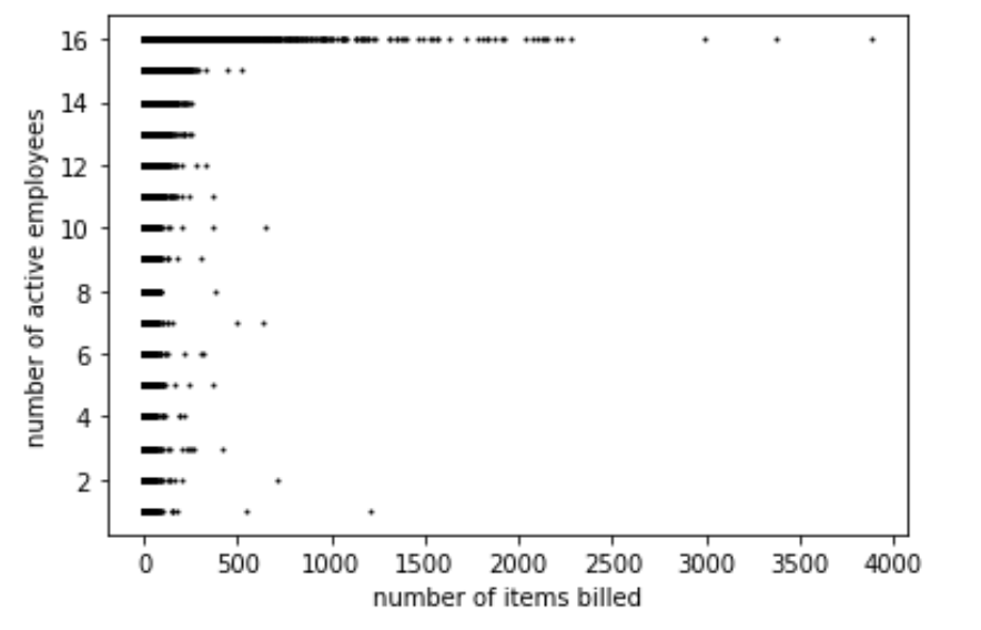
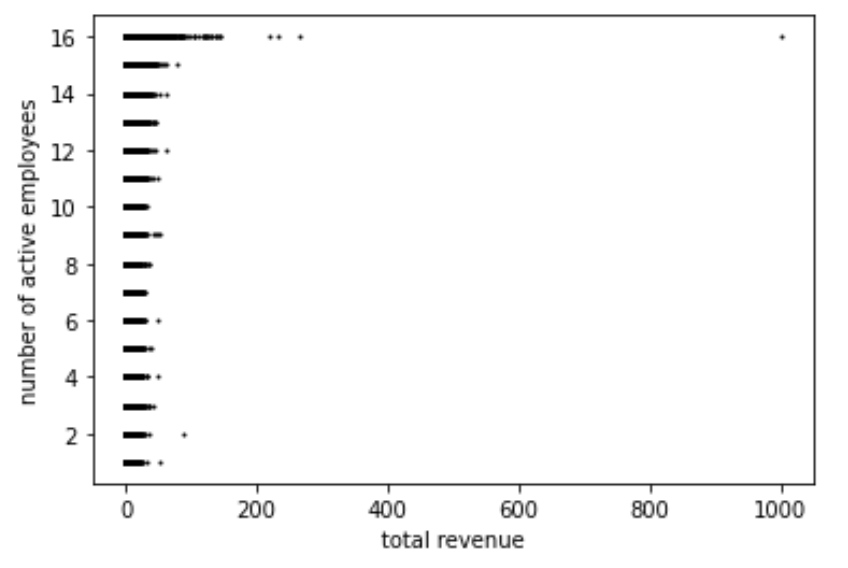
Figure 2 plots the number of active employees on the vertical axis with the number of items billed for payroll on the horizontal axis. The number of items billed is similar for groups 1 to 15, but it exceeds 500 for group 16. In other words, the number of items billed is much larger when the number of active employees is among the highest. (we do not know the exact values since the feature is binned into groups.) The same thing happened with total revenues, as shown in Figure 2. The vertical axis is the number of active employees binned to groups, and the horizontal axis represents the total revenue, which is a normalized numerical variable. The range of total revenue is uniform for groups 1-15, and once the revenue exceeds 100, it is likely to be a member of group 16.
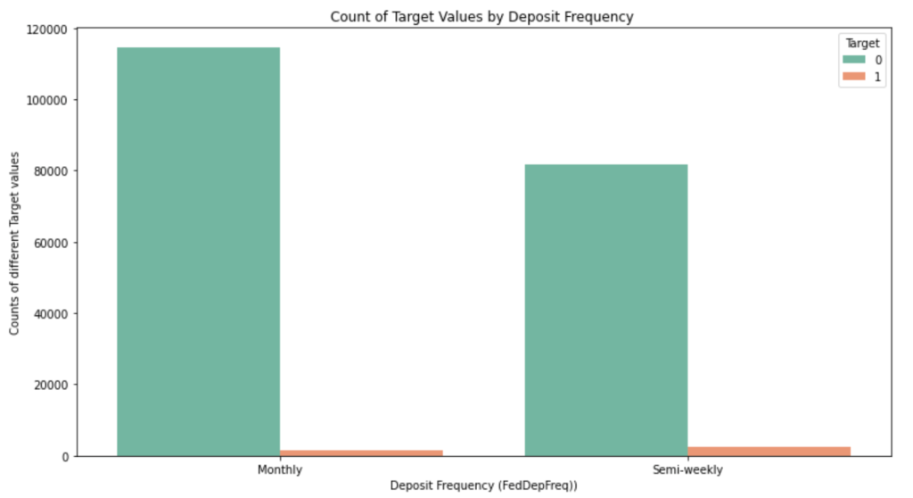
Figure 4, on the other hand, reflects the relationship between FedDepRreq (deposit frequency) and the target variable. It shows that clients who make a deposit monthly are less likely to add the 401(k) services since the number of total cases of label “monthly” is larger, but the number of labels 1 is smaller.
3.2 Data Imbalance
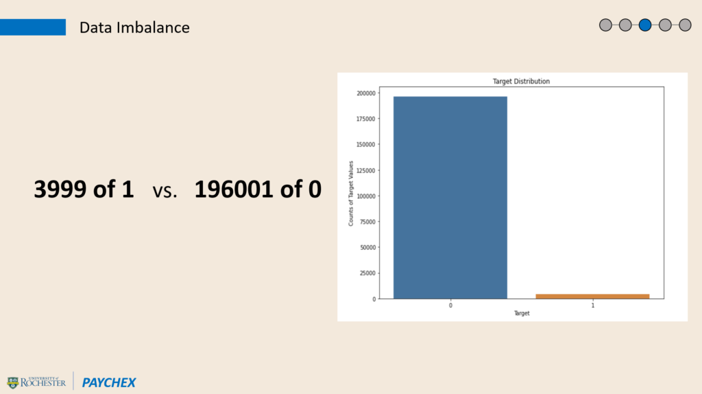
The dataset has an extremely imbalanced dependent variable. Figure 5 visualizes the distribution of Target, where the rate of label 1 is only 2%: the dataset contains only about 3999 examples of class 1, while there exist 196,001 cases of label 0. The imbalanced problem might cause an overfitting issue when the predictive models overfit with label 0 and miss many potential 401(k) clients. Thus, reducing the difference between the number of these two values has been a crucial point.
4. MODEL DEVELOPMENT
4.1 Oversampling and Undersampling
To support the project objective of predicting whether a client will buy 401(k) services or not, we propose to apply different classification methods and build a decent model. First, to avoid models from overfitting, we work on the imbalanced target problem.
There are two practical approaches to adjust the target distribution: oversampling and undersampling. After trying different methods of these two approaches (SMOTE, ASASYN, e.g.), random oversampling and random undersampling stand out to be the more appropriate ones.
- Random oversampling means we supplement the data with copies of randomly selected samples from minority class [4], which is label 1 in this case, as the project aims to have more examples in the minority class.
- On the other hand, random undersampling randomly removes samples from the majority class [4], which is target “0” here, as it hopes to decrease the number of samples in the majority class.
After splitting data into testing and training sets by a ratio of 3:7, we tried different strategies of oversampling and undersampling on various classification methods, including Binary Logistics Regression, K Nearest Neighbors, and Random Forest. Under the suggestion of the Paychex team, we also tried Boosted Random Forest, Lasso and Ridge regression. We agreed with our sponsor that accuracy is not crucial in our case, and we value more on precision and recall for label 1. It turns out that Random Forest has a significantly better result than other methods, which means there is no need to spend more time on other models. As a result, we followed our sponsor’s suggestion to focus on Random Forest.
4.2 Random Forest
Random Forest is a collection of decision trees, usually trained with a bagging method.[5] The randomness comes from its random trees built from random samples and randomly selected features at each node. The bagging method, also called bootstrap aggregating, is a machine learning ensemble meta-algorithm designed to improve stability and accuracy.[5] The randomness and the bagging method reduce variance and help avoid overfitting as it decreases the chance of getting stuck at a local maximum.
4.3 Model Building Process
We applied different oversample-undersample criteria with random forest, including undersampling only, oversampling only, and a different ratio of combining oversampling and undersampling. Besides, we tried training on selected subsets of features to improve the overfitting issue, but it turns out that training with all features has the best result. Figure 6 is the best combination we got.
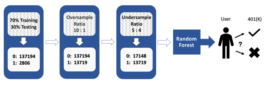
- Split the dataset by 70% for training and 30% for testing. Numbers at the bottom record the number of samples in label 0 and 1.
- Oversample copies of existing label 1s, until the number of labels 1 is 90% less than label 0, resulting in a 10 to 1 ratio.
- Use undersampling to randomly remove cases of label 0, until label 0 is 20% more than label 1, resulting in a 5 to 4 ratio.
- Build the predictive model using Random Forest to classify clients into good candidates and poor candidates, and measure model performance based on the testing set.
5. PERFORMANCE AND RESULTS
5.1 Performance
Figure 7 shows the classification report of the Random Forest model, which is the best result among all attempts.
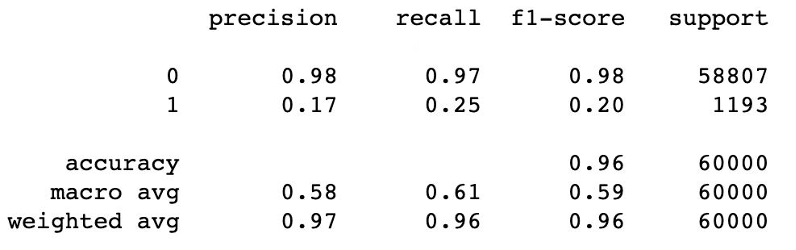
To support project vision, we focus on precision and recall for label 1. Precision attempts to answer on what proportion of positive identifications is actually correct.[6] It is calculated by dividing the number of true positives by the sum of true positives and false positives. In this case, the precision of class 1 tells us that of all clients who the model predicts to buy the 401(k), how many of them will actually add the services. Therefore, we want the precision to be as high as possible. Recall, on the other hand, attempts to answer on what proportion of actual positives is identified correctly.[6] It is calculated by dividing the number of true positives by the sum of true positives and false negatives. We also want the recall to be high because the higher the recall, the lower the chance that we miss a 401k client. We also calculate the lift score, which measures the effectiveness of our model. A higher lift score is better.
5.2 Result Analysis
In this model, the precision for label 1 is 0.17, recall is 0.25, and the lift score is 8.52. Precision tells us that using this model, in around five clients that Paychex reaches, one of them will buy the 401(k) services. Recall states that Paychex will successfully get 25% potential clients of 401(k) services based on this model. The lift score represents that classification we made is 8.5 times better than randomly generated classification. We agreed with our sponsor that the result is satisfactory for a marketing setting.
6. MODEL EXPLAINERS
6.1 LIME
LIME stands for Local Interpretable Model-agnostic Explanations. It is an algorithm implementing local surrogate models, which are trained on the black box model to give predictions. LIME only has local fidelity. It cannot give global interpretations, but it is very fast to run. [7]
The process includes five steps [8]:
- Select the instance which you want to explain.
- Generate a new dataset permuting data samples and get the corresponding predictions from the black box model.
- Weight the created samples by the proximity to the instance of interest.
- Train an interpretable model (random forest, lasso, e.g.) on the new dataset.
- Explain the instance based on the local mode.
6.2 SHAP
SHAP (Shapley Additive explanation) by Lundberg and Lee [9] is an approach to explain machine learning model outputs, leveraging the Shapley values from game theory. A Shapley value is the “average marginal contribution of a feature value across all possible coalitions.” [8] It tells the contribution of a variable to the difference between a particular prediction and the average model output. Because Shapley values compute all possible predictions for an instance using all possible combinations of input features, SHAP is exhaustive and guarantees better consistency and accuracy than previous methods, but it is also time-consuming. The SHAP Python library helps to speed up the computing time using approximations and optimizations. In this project, we apply the tree explainer because it runs fast on random forests.
7. ANALYSIS OF EXPLAINERS
7.1 Local Explanations
One of the project goals is to see why the model says a particular client is going to add the 401(k) services; therefore, we picked two examples to explain. Besides, since the model predicts many more cases with Target equals to 0 but the Paychex team wants to focus more on clients who are likely to buy the 401(k), we only showed examples which are correctly predicted to have Target equals to 1.
7.1.1 Example I
Figure 8 shows the LIME results of the first example. First, the model predicts the probability of this client buying the services is 64%. Second, features on the left side have decreased the probability while features on the right increase the probability. It says that having no revenue of Product11 and Product07 decreases the probability, but the client is still likely to add the 401(k) thanks to contributions of features including Product19, Product14, Product09, etc. Payroll_Frequency_5 <= 0.00 means the payroll frequency does not equal to 5, and checking through the dataset, the payroll frequency is 2 for this client. ActEEsPct_Binned_1 <= 0.00 means that the percent of active employees is not of the first binned group but is of binned group 4.
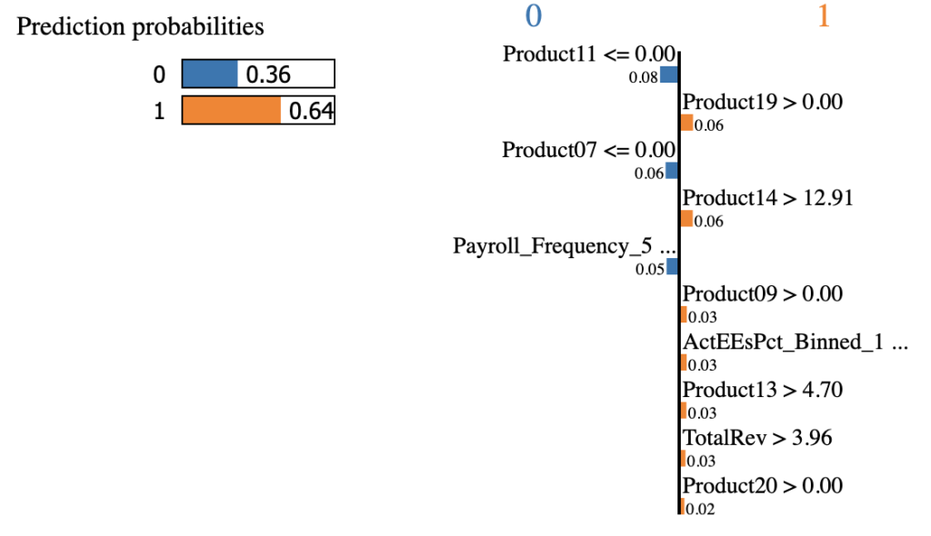
(features that did not display fully:Payroll_Frequency_5 <= 0.00, ActEEsPct_Binned_1 <= 0.00)
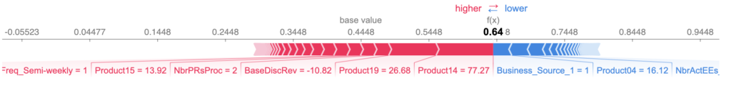
Figure 9 gives us the results from SHAP. It gives us a base value and an output value. The base value is the average output over the training dataset in log-odds because we have a classification model, and the output value is the predicted probability for this instance. Features pushing the prediction higher are shown in red, those pushing the prediction lower are in blue, and the length of the arrow measures the magnitude of effect. The graph says that the biggest effect is Product14. Product 9 is the second, which means that these relatively high revenues have positive impacts on the output. Business_Source_1 equals to 1 and Product04 has decreased the probability. In other words, having some revenues of Prodcut04 actually drives the probability lower.
7.1.2 Example II
Figure 10 is how LIME explains the second example, which has a probability of 77%. Product11 is the absolutely top driver. This client has no revenues on Product19 nor Product14, so they decrease the probability. Just like the first example, ActEEsPct_Binned_1 <= 0 increases the probability, while Payroll_Frequency_5 <= 0.00 drives the percent down.
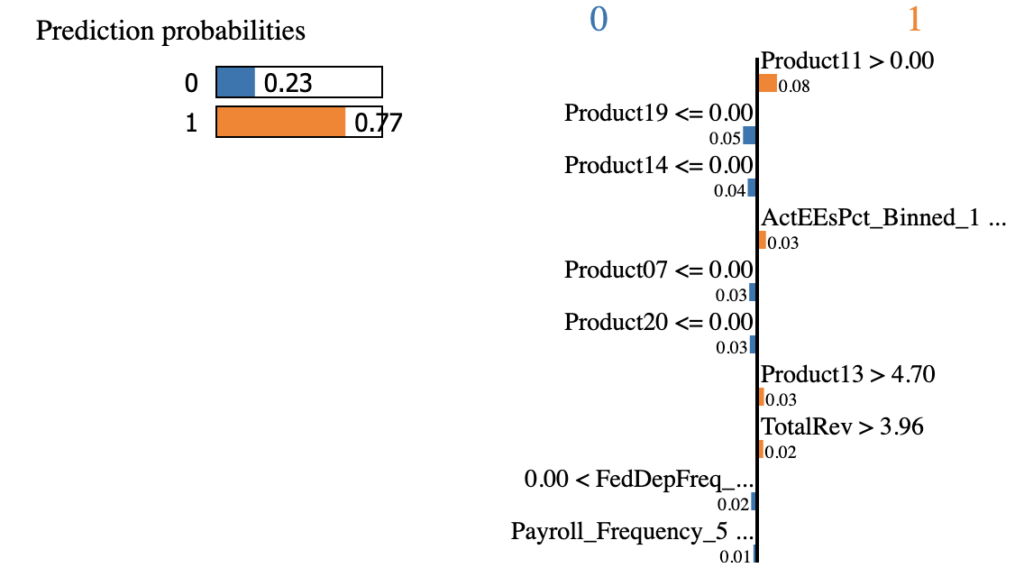
(features that did not display fully: ActEEsPct_Binned_1 <= 0.00, 0.00 < FedDepFreq_Monthly <= 1.00, Payroll_Frequency_5 <= 0.00)
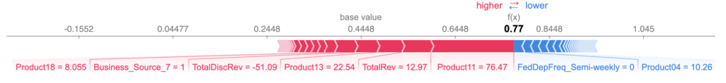
Figure 11 is the explanation for the second example given by SHAP. Product11, again, has the biggest positive impact, followed by TotalRev, Product13, etc. On the other hand, FedDepFreq_Semi-weekly = 0 (deposit frequency is monthly) and Product04 = 10.26 (revenue of product04 is 10.26) decrease the output. Product11, 13, and TotalRev are presented in both explanations.
7.1.3 Comparison
The results of LIME and SHAP on the same cases have some in common but also some differences. The first difference is obviously the different features, especially when explaining features that have negative impacts on the prediction. Another finding is that LIME tends to put the same features with different values on two sides. For example, in the first case, LIME states that Product11 <= 0.00 (no revenues of Product11) drives the probability down. While in the second case, it classifies Product11 >= 0.00 as the positive influencer. The same thing happened with Product19, Product14, and Product20. However, SHAP does not show the same tendency. But more instances are needed to make a firm argument about this difference.
One possible explanation for the different results generated by LIME and SHAP is to look at their definitions and training processes. LIME creates a surrogate model locally around the unit whose prediction you wish to understand. Thus, it is inherently local, and it may be biased because it only looks at the neighborhood. While Shapley values ‘decompose’ the final prediction into the contribution of each attribute and might be the only method to deliver a full explanation.
7.2 Global Interpretations
Since SHAP takes all possible coalitions into account, it can give out global explanations using aggregations of Shapley values.
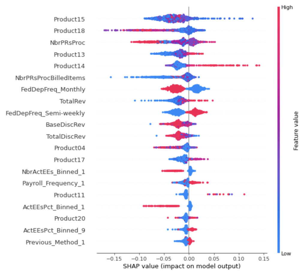
Figure 12 shows the impact of features on the output. The computing time for the whole training dataset is too long, so we only used 1000 examples of the training data to generate this plot. Here, the different colors refer to different values: redder means high and bluer means lower.
Things shown by the graph:
- High revenues of Product14 will increase the probability, but a small range of Product14 corresponds to a large range of output.
- Higher total revenues and Product13 revenues are also likely to raise the likelihood.
- In most cases, having a semi-weekly deposit frequency leads to a positive probability.
- For Product11 and Product17, having relatively high revenues has a positive impact, and Product11 has a bigger impact.
- When Previous_Method_1 equals to 1, the influence is likely to be positive.
- According to NbrActEEs_Binned and ActEEsPct_Binned, smaller numbers of active employees and smaller percent of active employees both result in negative probabilities.
- And for Product 18, higher revenues indeed drive the probability lower, reflecting a negative relation.
- Having low revenues of Product 15 is likely to increase the probability, but it may also lead to low probability, because the blue dots are also shown in the left side of the axis.
8. CONCLUSION AND FUTURE WORK
This paper employs the dataset from Paychex and aims to predict whether an existing client is going to add the 401(k) services and give model explanations. After comparison and adjustments, the Random Forest model has shown to be the most promising considering precision, recall, and lift score. Thus, the Paychex team could put new data into the model and call clients based on the generated results. LIME and SHAP are applied and compared to explain specific instances, and SHAP might be the more consistent one. SHAP also gives out global interpretations using part of the training data. The Paychex team could dig more into the properties and information of those influential features to see why they increase or decrease the probability, since the new findings might be useful when organizing a marketing campaign. Besides, when they want to promote the 401(k) services, they can call clients based on the global explanations to enhance their efficiency and chance of hitting. For instance, they could call clients with high revenues of Product14 first.
Nonetheless, the model is trained on repeated samples and the global interpretation is based on part of the data, so generality should be examined when the models are applied for other applications. Further research would involve other machine learning algorithms and techniques which this paper has not tried; getting more data of the minority class would also improve the model performance; if there is more time or better computing power, SHAP could be trained on the whole dataset to improve accuracy and exhaustiveness of global analysis.
Acknowledgments
We would like to thank Michael Lyons, Val Carey, Jing Zhu, Satish Prabhu, Professor Ajay Anand, and Professor Pedro Fernandez for helpful suggestions and feedback.
References:
- What Is a User Persona? User Persona Definition, Benefits and Examples. (n.d.). Retrieved December 13, 2020, from https://airfocus.com/glossary/what-is-a-user-persona/
- How our Solutions Work. (n.d.). Retrieved December 13, 2020, from https://www.paychex.com/how-paychex-works
- Paychex, Inc. Reports Fourth Quarter and Fiscal 2019 Results; Total Revenue Growth of 12% to $3.8 Billion for the Fiscal Year. (2019, June 26). Retrieved December 13, 2020, fromhttps://www.businesswire.com/news/home/20190626005088/en/Paychex-Inc.-Reports-Fourth-Quarter-and-Fiscal-2019-Results-Total-Revenue-Growth-of-12-to-3.8-Billion-for-the-Fiscal-Year
- Brownlee, J. (2020, January 15). Random Oversampling and Undersampling for Imbalanced Classification. Retrieved December 13, 2020, from https://machinelearningmastery.com/random-oversampling-and-undersampling-for-imbalanced-classification/
- R, A. (2020, May 23). A Simple Introduction to The Random Forest Method. Retrieved December 13, 2020, from https://arifromadhan19.medium.com/a-simple-introduction-to-the-random-forest-method-badc8ee6c408
- Classification: Precision and Recall | Machine Learning Crash Course. (n.d.). Retrieved December 13, 2020, from https://developers.google.com/machine-learning/crash-course/classification/precision-and-recall
- Ribeiro, M., Singh, S., & Guestrin, C. (2016, August 09). “Why Should I Trust You?”: Explaining the Predictions of Any Classifier. Retrieved December 13, 2020, from https://arxiv.org/abs/1602.04938
- Molnar, C. (2020, December 07). Interpretable Machine Learning. Retrieved December 13, 2020, from https://christophm.github.io/interpretable-ml-book/
- Lundberg, S., & Lee, S. (2017, November 25). A Unified Approach to Interpreting Model Predictions. Retrieved December 13, 2020, from https://arxiv.org/abs/1705.07874
Featured Image: Watson, L. What Should I Do With My 401k? (n.d.) Retrieved May 10, 2021, from https://dreamfinancialplanning.com/blog/what-should-i-do-with-my-401k