Team
- Bowen Jin
- Zeshu Li
- Hanrui Liu
- Tianbo Liu
Mentor
Professor Ajay Anand
Dr. Preston Countryman
Sponsor
Corning Inc. – Data Science & Intelligence (DSI) Team
Abstract
Corning wants to develop a deep-time-series model to perform accurate customer-level demand forecasting using daily purchasing data. The goal of this project is to predict the revenue income in a given time period and predict quantity demand from selected products. To deliver against these goals, our team developed a basic time series model using the Prophet model to perform revenue forecasting, which served as a benchmark for the deep learning model. Our team then went through a series of re-sampling, feature engineering, and hyper-parameter tuning in preparation for the deep learning model. Finally, our team developed a time series-oriented, deep-learning model using LSTM to perform periodic revenue forecasting. The model eventually outperformed the baseline model evaluated by RMSE in multiple set periods. In addition, our team also developed an RFM analysis combined with clustering analysis to provide distributor and customer segmentation and other business insights.
Introduction
It is well known that any manufacturing company that wants to succeed must have accurate demand forecasting. It guarantees that businesses have the appropriate quantity of inventory and can react quickly to changes in demand. In recent years, Machine learning has emerged as a crucial element of accurate demand forecasting. Machine learning algorithms can examine previous sales patterns to determine future trends in demand forecasting. Based on this information, the algorithms will provide an appropriate model. The forecasting model improves in precision as more data are gradually added to the system. Demand forecasting using machine learning algorithms has completely changed how firms prepare for the future. The ability of businesses to estimate sales trends and make educated pricing or inventory management decisions can be greatly improved by combining conventional approaches with contemporary AI technology like machine learning.
Our client, Corning Inc., is a large manufacturing company with over 60,000 employees worldwide. While mainly manufacturing glass panels, funnels, liquid crystal display glass, and projection video lens assemblies for the information display market, Corning has coupled its unmatched expertise in the fields of glass science, ceramics science, and optical physics with strong manufacturing and engineering skills for nearly 170 years. In this project, our model aims to help Corning in better supply chain management and cost saving, improving targeted sales efforts, and reducing manual efforts in forecasting.
Dataset
Dataset Information
Given by our sponsor, Corning Inc., we have a dataset containing 72,716 rows with 11 columns regarding Corning’s customer purchases. The dataset recorded all the transactions made from 2012 to 2020, and one row in the dataset represents a single transaction made from a buyer to Corning.
Data Preprocessing
Our team performed two rounds of data manipulation in preparation of the models. We first did a preliminary round of data preprocessing which checks missing values, creates needed variables, and transforms the dataset in a daily format. Then in the model section, we will discuss the feature engineering process that is essential to our models.
Through our data preprocessing, we found that the ‘customer’ column has nearly 40\% of missing data, which prevents us to create customer-level predictions in our models, while other important columns like ‘quantity’, ‘unit_price’, and ‘std_cost’ columns have no missing values.
We also calculated the revenue/sales of each transaction by taking the product of the ‘quantity’ and ‘unit_price’ variables.
In addition, we converted the ‘date’ column from string datatype to datetime datatype and aggregated the dataset by date, which gives us over 1400 individual days and their daily revenue from 2015 to 2020. However, by looking at the dates from the first couple of days, we realized that the dates are only weekdays from each week, and the weekend dates are skipped in the dataset. Therefore, we decided to add the missing days on the weekend and their date in the ‘date’ column, and add everything else as 0, since there are no sales. We used the resampling function from the pandas package to add the missing days on the weekends.
Exploratory Analysis
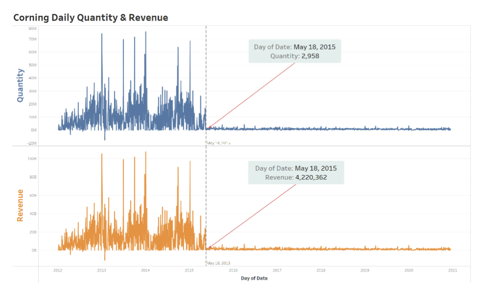
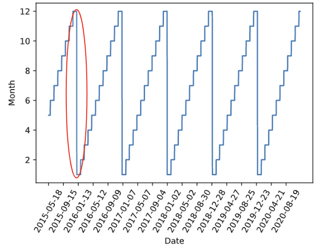
After aggregating our dataset by date, we can now take a look at the behavior of our main variables, ‘revenue’ and ‘quantity’ on a time-series level. We found that due to the business strategy and client contract situation from Corning, both the daily quantity and daily revenue dropped drastically after May 18 of 2015. In order to capture the latest trends and make the best prediction, we decided to only use data after May 18 of 2015 in our models, which is the most recent and seems stable at least for the past few years.
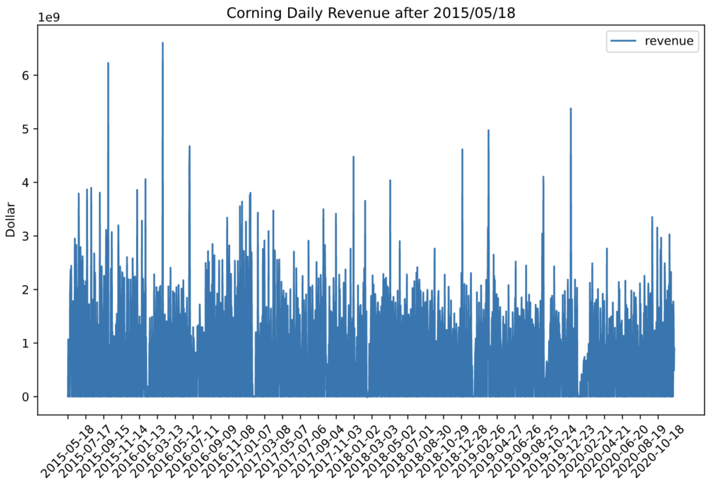
As we take a look at the time-series plot of revenue after May 2015, we can see that the revenue is showing no obvious trends, and the subtle oscillation shows evidence of some seasonality. After conducting an ADF stationary test, the very low p-value (lower than 0.001) proves that the data is stationary. No future data manipulation is needed to fit the data into a stationary state such as first-order differentiation and exponential smoothing.
Feature Engineering
Select Top Selling Products
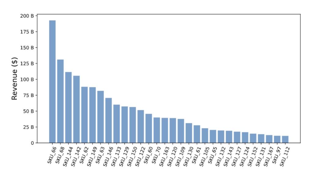
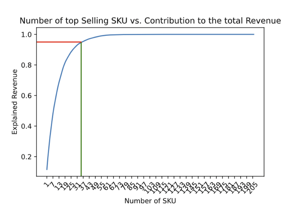
So far our model only contains the time-series variable ‘date’ and the targeted variable ‘revenue’. We want to include more information in the model. Therefore, we want to include the ‘SKU’ variable from the original dataset in our deep learning model as dummy variables. However, there are over 200 distinct products being sold in our dataset. After plotting a bar chart that shows the total revenue of each product in the time frame ranked from high to low, we can see that a small group of products contribute toward most of the sales. We then decided to include only a few top-selling products’ daily revenue which contributed toward most of the revenue income, as adding these helps the model to make predictions while we don’t need to worry about overfitting issues. We can see that the intersection point indicated that the top 35 popular SKUs contributed toward more than 90\% of the sales after 2015. We can then select these top 35 products and make them into dummy variables and feed them into our models later. Our model enables users to input their desired level of revenue being explained by the top-selling SKUs and creates dummy variables according to the users’ decisions.
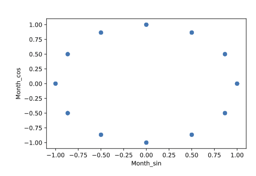
Convert Weekday and Month into Cyclic Patterns
In order to include more data in our models, we decided to feed in the ‘month’ and ‘weekday’ two variables each created using the ‘date’ variable from the original dataset. However, the LSTM model does not recognize 1-7 and 1-12 as a complete cycle, it just identified them as a level categorical variable in integer form, and there will be a numeric gap between 1 and 12 and 1-7 while in reality, January is right after December. To train the model using these variables as a cyclic pattern, we converted 1-7 and 1-12 as cosine and sine scores, as shown in the example of months. By doing so, we can let the deep learning algorithm know that features such as month and weekday occur in cycles.
Extract the Number of Unique SKU, Product Group 1, and Product Group 2 being sold each day
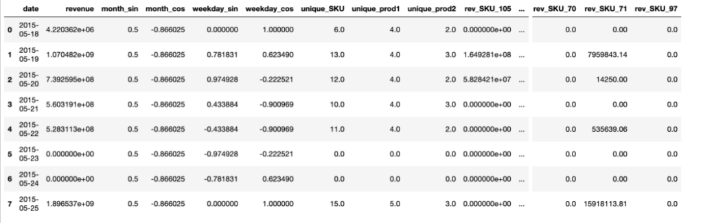
Our goal was to enhance the level of detail in our dataframe, so we decided to record the daily count of distinct SKUs, product group 1, and product group 2 being sold. And, the final dataframe has 2035 rows and 46 columns. Here’s a final look of our dataframe.
Model Development
The goal of this project is to build a deep-time-series model to predict future revenue and quantity demand for Corning Inc. For this purpose, we first chose a well-known time series model, the Prophet from Facebook Inc. (Meta Platform, Inc.), as our baseline model to use its result to compare the performance of the model we finally designed. Then, after resorting to some published literature, we developed a deep learning time-series-oriented model using LSTM (Long Short-term Memory Networks) to perform future revenue and quantity forecasting.
Prophet
Prophet is a time-series forecasting model developed by Facebook’s Data Science team. We chose it as our baseline model because it is an open-source tool that is widely used in the industry for its simplicity and ability to handle complex data patterns. The Prophet model would analyze the revenue data and identify any trends, seasonality, and other factors that may affect revenue. It would then use this information to make predictions for future revenue.
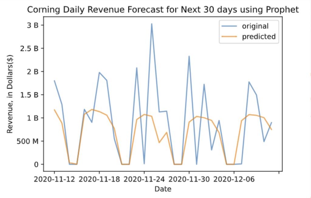
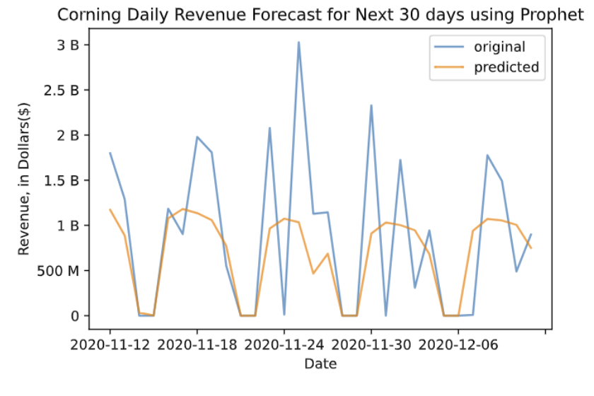
In this case, we built a univariate forecasting model, using the past revenue data as our only X variable to predict the future revenue level. We used the last 30 days as our testing set and the rest of the data as our training set. The graph below is the forecasting result for the testing set. The blue line represents the true values and the orange line represents the forecasting values. From the evaluation metric we chose here, the RMSE value is about $0.7 billion, which means the average difference between the true value and the predicted value is $0.7 billion. The error would be large when we see this number alone, but if we compare it to the range of our dataset, which is $4 billion, the number may seem acceptable. Although our original dataset does not possess a clear weekly pattern since it only contains transaction records on weekdays, after filling in the missing weekend data, we gave the dataset a weekly pattern, as it has a high revenue level on weekdays and low or no revenue on weekends. From the image below, the predicted values possess a clear weekly pattern with a smooth, almost bell-shaped trend, which is not too fit to the actualities because it does not quite catch the fluctuating and high revenue levels.
LSTM
LSTM is an RNN variant that addresses the issue of the gradient vanishing problem in conventional RNNs. Its particular structure enables it to choose what to retain or discard from the input data over extended timeframes, making it a suitable option for processing sequential and time-series data. We chose to use this model in our project from the past scholars’ and practitioners’ experience dealing with time-series problems.
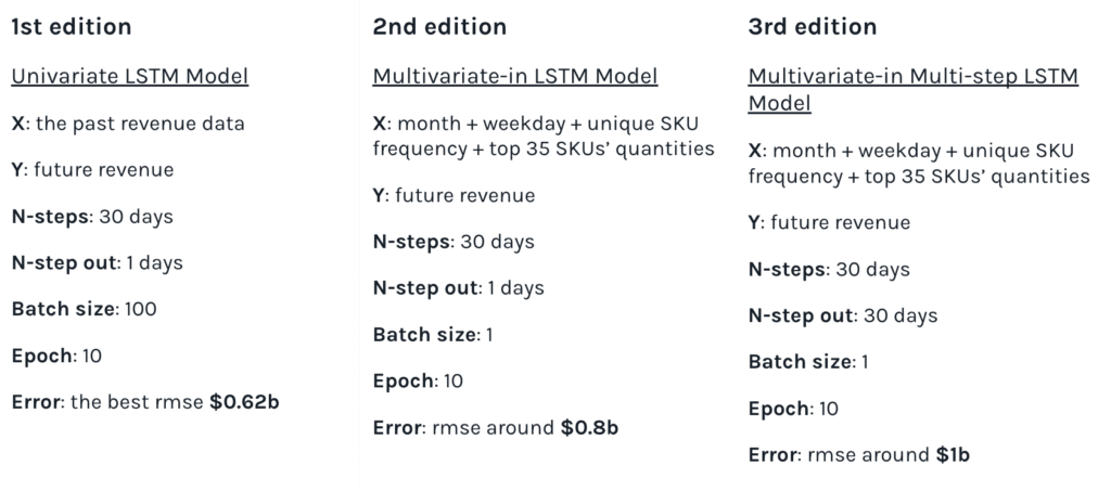
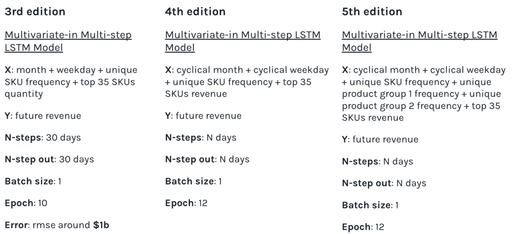
Our own deep learning modeling process has gone through different versions, starting with a single-variable forecasting model and ending with a multivariable forecasting model that can achieve an arbitrary number of days forecasts, during which we have done a lot of adding and tuning of input values and model parameters. The image below shows a clear explanation of our model iteration.
Parameter Tuning
As we continued to iterate the model, we also tuned the model at the same time. We tried to fine-tune all the changeable parameters, which include the activation function, number of layers, number of nodes in each layer, the type of each layer, number of batch sizes, and number of epochs. However, among all other activation functions, we found that “Relu” and “Selu” performed better. We also tried adding either more nodes or layers to our network, but the model performance hardly improved and might even worsen. So, at that stage, we decided to focus on further fine-tuning the in and out parameters, which are the N-step and N-step out, along with our activation functions.
Performances and Results
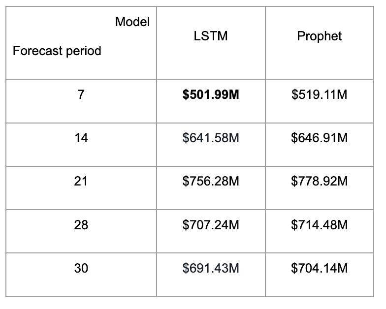
From the table below, we can see that by evaluating the RMSE value, the LSTM model consistently outputs better performance than the Prophet Model. The lowest RMSE value we achieved is $501.99 million dollars, predicting the revenue of the next 7 days. After comparing the performance of our LSTM model and the Prophet model in multiple forecasting periods, we can confidently say that we have reached our goal to build a deep-time-series model that can outperform the baseline model.
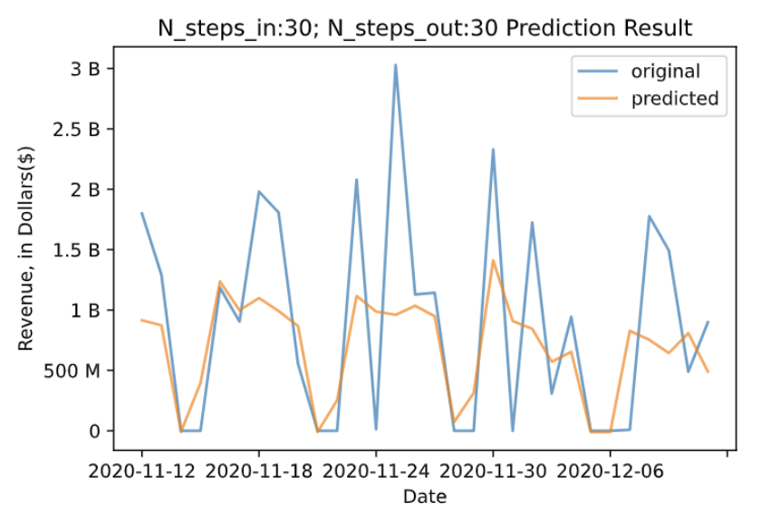
To make sure that the LSTM model does a better job than the Prophet model, we plotted the predicted curve versus the actual revenue curve for both models given the 30-day forecasting period. We can see that the LSTM model does a better job of predicting the sudden increase and decrease and capturing the detailed peaks within the 30-day period. The visualized comparison between the model outputs gives more assurance that the LSTM model fits better.
Conclusion & Next Steps
In this project, we started with a series of data manipulation and exploratory analysis, where we selected appropriate segments from the dataset, created variables for model inputs, and added cyclical patterns to certain variables for appropriation. Then we created a baseline model using Prophet, which set a bench score for our deep learning model. After an extensive series of model development and hyper-parameter tuning, our deep learning model, LSTM, achieved a low RMSE of \$501.99 million dollars given a 7 days forecasting period. Meanwhile, our LSTM model perform consistently better than the Prophet model in the 5 different forecasting periods that we tested. In addition, we conducted an RFM analysis that provides distributor and customer segmentation and other business insights.
Although we reached our goal for this project, our error value is still quite large, and the predicted curve is pretty conservative at predicting the peaks in the dataset. In the future, there are a lot of potential improvements that can make the model output better performances. One example is to include more variables that reflect Market Trends, Economic Indicators, and Industry Data such as GDP, changes in inflation rates, production/inventory levels, and other variables that explain potential revenue change.
Reference
[1] Aaina Bajaj. RFM analysis for successful customer segmentation using python. https://aainabajaj39.medium.com/rfm-analysis-for-successful-customer-segmentation-using-python-6291decceb4b,
Nov 2020.
[2] Jason Brownlee. How to develop LSTM models for time series forecasting. https:
//machinelearningmastery.com/how-to-develop-lstm-models-for-time-series-forecasting/,
Aug 2020.
[3] Nicapotato. Keras timeseries multi-step multi-output. https://www.kaggle.com/code/nicapotato/
keras-timeseries-multi-step-multi-output/notebook, Apr 2020.
[4] Andrich van Wyk. Encoding cyclical features for deep learning. https://www.kaggle.com/code/
avanwyk/encoding-cyclical-features-for-deep-learning, Sep 2022.
11