
Photo: Ayers Saint Gross
Supervisors
Ajay Anand
Pedro Fernandez
Department of Data Science at University of Rochester
Sponsors
Alexander Pfadenhauer
Tim Vann
University of Rochester Utilities
Project Vision & Goals
UR Utilities and Energy Management hopes to improve the efficiency of chilled water production through predictive modeling.
Our team hopes to provide a package of models which can accurately predict, within 500 tons.
1. Daily max CHW demand ( 4-day lookahead)
2. Time of daily max CHW demand
3. Hour by hour forecast of max CHW demand (24+ hour lookahead)
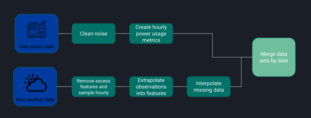
Description of Datasets
Our first dataset includes Time series data of power for each chiller, spanning March 1, 2019 to March 1, 2021; interpolated in 1-minute intervals. This dataset contained occasional negative power values and outliers which were later zeroed out or removed during data cleaning.
The second dataset was weather data pulled from the National Oceanic and Atmospheric administration (NOAA) which gave hourly measurements sporadically. To match power data that was interpolated hourly, we used weather data observation at the 54 min mark as it contained consistent observations. This weather dataset also required a lot of data cleaning because there were multiple instances of strings mixed with integers.
Data Cleaning
Exploratory Data Analysis
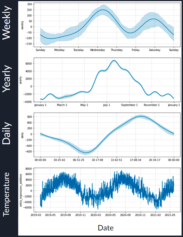
For our initial exploratory data analysis, we performed seasonal decomposition on a variety of levels to get a better understanding of the data we will be working with. In the above graph we extracted the weekly seasonality where we can see peaks in the middle and end of each week. We also extracted the yearly seasonality with an obvious spike in the summer. The daily seasonality shows a dip in the morning with a spike in the evening. Finally, we display the temperature fluctuations throughout the year as we believe this will have a significant impact on our modeling.
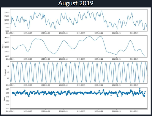
Next we zoom into a singular and highly variable summer month (August 2019) and again perform a seasonal decomposition. The top row shows how the total power output fluctuates throughout the month. The second row shows us the moving average trend minus the daily seasonality, which can be seen extracted on the third row. The final row shows the error residuals than cannot be explained by just the trend and daily seasonality components.
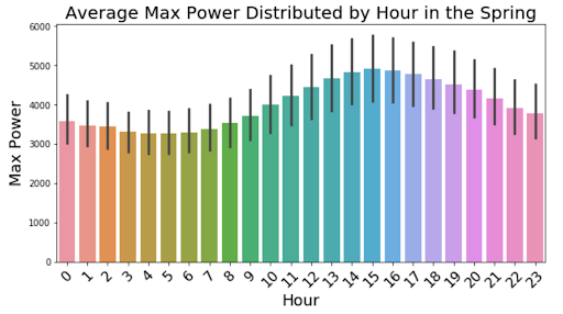
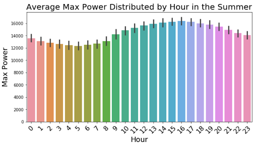
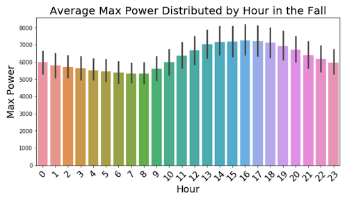
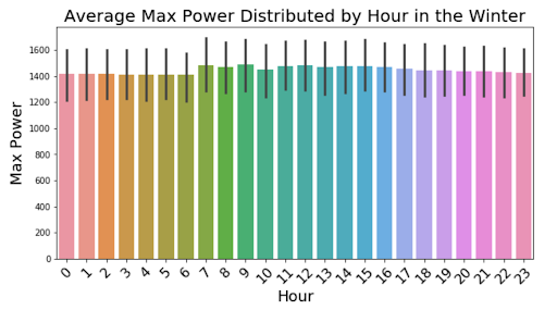
For further insight into how the power changes on a day to day basis, we split the mean power output for each hour by season with a 95% confidence interval and displayed them in the graphs above. These graphs show dips in the morning and peaks in the afternoon for the Spring, Summer, and Fall seasons. The Winter season remains fairly uniform throughout the day.
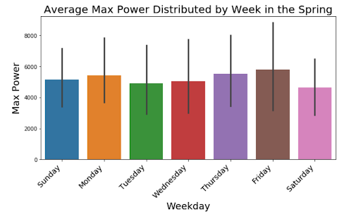
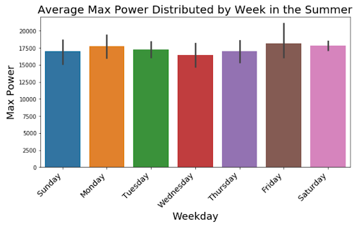
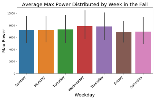
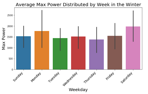
Next we want to look at how the power changes throughout the week for each season. These graphs offer alternative information to the weekly seasonality that was displayed in our first seasonal decomposition. There seems to be consistent peaks on Monday and the end of the week for all seasons except the Fall, where we can see a clear increase in the middle of the week. It is interesting to see how the different seasons can reflect different weekly seasonality of power outputs.
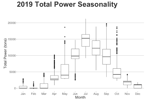
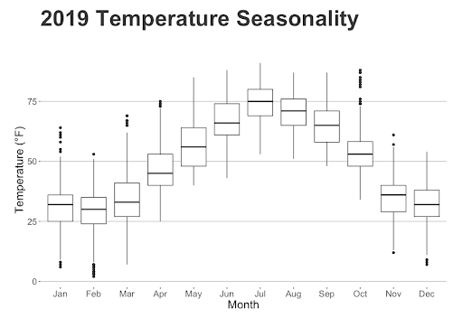
We wanted to revisit how temperature and power change throughout the year with a side by side boxplot comparison. In the year of 2019 we can see how there is a clear correlation between the two trends, with both steeply increasing in the summer and decreasing in the winter.
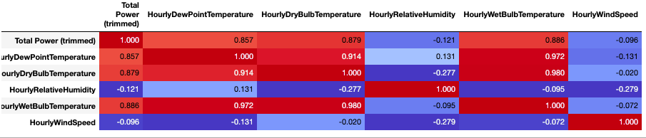
Further looking into the temperature, we created a heatmap of the weather variables that we would go on to use in our modeling. We can see that there are fairly strong correlations between some of the features and we took this into account when using them in our models.
Modeling
To achieve our three project goals, we created two separate models. One would provide an hourly forecast of the next 12 hours to predict the current day’s maximum power output and the time it would occur. The other model would forecast the daily max for the next 4 days to predict which day would have the highest.
Predicting Daily Max
Initially we looked at various machine learning models as well as traditional SARIMA models to predict the daily maximum power output in tons. After testing with each type of model and adjusting parameters, such as the number of days in the past the model uses for prediction, we found that the Gradient Boosting and Random Forest models had the best performance. We decided to use Gradient Boosting because of its quantile feature.
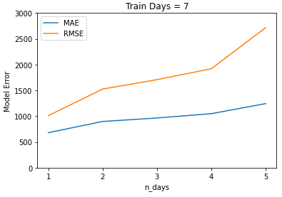
| Number of Days in to the Future | Mean Absolute Error |
|---|---|
| 1 | 680.7 tons |
| 2 | 898.1 tons |
| 3 | 965.5 tons |
| 4 | 1049.3 tons |
| 5 | 1244.6 tons |
Our testing found that including the weather and power data from 7 days before the prediction yielded the best results.
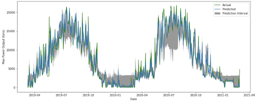
Gradient Boosting Daily Max Results:
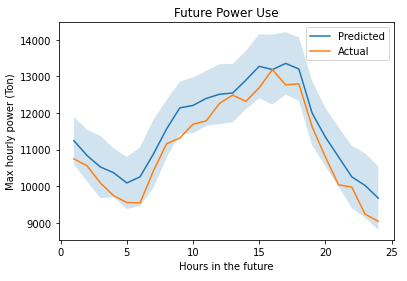
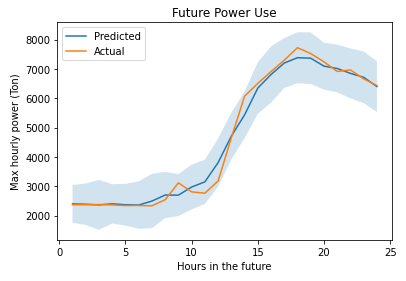
Hour by Hour Forecast
With this approach we only created a machine learning model. For each hour, we captured a 24 hour lookback of max power, dry and wet bulb temperature, as well as a 24 hour lookahead of dry and wet bulb temperatures to serve as our “forecasted” weather data. Using this, we generated two time series features to help describe the trend: exponentially weighted mean and average difference. Once we had all our features, we performed sine and cosine transformations on the daily, weekly, and monthly seasonality. One model was created for each future hour prediction.
| Model | Avg. RMSE over 12 hr Prediction (tons) | |
|---|---|---|
| Linear Models | Linear Regression | 962.3 |
| Non-Linear Models | KNN | 1251.8 |
| SVR | 3726.5 | |
| Decision Tree | 756.81 | |
| Ensemble Methods | AdaBoost | 1716.3 |
| Random Forest | 467.91 | |
| Extra Trees Regressor | 388.0 | |
| Gradient Boost | 648.73 |
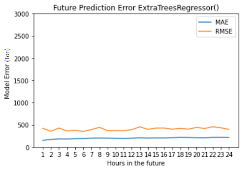
After testing several models, Extra Trees had the best performance.
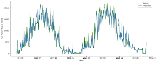
After tuning the Extra Trees model, we were able to predict future power usage within approximately 800 tons (95% confidence level) and our average RMSE was 399.73 tons
Conclusion
While our models didn’t quite reach the 500 ton MAE benchmark we were aiming for, we were able to get reasonable accuracies for each desired forecast of maximum power output (4-day daily max, current day’s hourly max, and time of current day’s max) within reasonable accuracy.
Acknowledgement
Thank you to Alex and Tim for sponsoring us and working to acclimate us to the data. Thank you to Professor Anand for giving us guidance and helping us work through challenges with our project.