Team
Steven Dai
Zachary Mustin
Uzoma Ohajekwe
Duy Pham
Sponsor
Vnomics Corporation
Matt Mayo
Mentor
Prof. Ajay Anand
Abstract
Our task is to predict imminent failures in Diesel Particulate Filters (DPFs) of truck trailers up to fourteen days before breakdown occurs and to identify critical indicators of DPF failures. Upon extracting daily trip records fourteen days before service dates and scaling the trip features as appropriate, we performed windowing and extracted useful features from each window using tsfresh, a Python Time Series library. After intensive model tuning, our highest Accuracy and Recall were 79.59% and 100.00% – using Random Forest. The strongest indicator of DPF failure is how long the DTC code SPN 3720 FMI 15 was active within each window. This code indicates the amount of ash accumulated in the filter. The more ash is accumulated, the more likely the DPF is to clog and fail.
Introduction
Modern diesel engines are equipped with Diesel Particulate Filters (DPFs), which filter out diesel particulate matter, or soot, from the exhaust gasses. If too much soot is built up and not removed, exhaust emissions become trapped in the engine – building up a large amount of pressure within. This pressure prevents the engine from operating efficiently and can potentially cause the engine to fail altogether. As the exhaust system becomes hot enough, the soot caught in the DPFs is oxidized and burnt off. However, sometimes DPFs become so clogged that regeneration fails to clean up the soot. In the worst-case scenario, this prevents the engine from operating, leading to costly roadside breakdowns.
Thus, our goal in this project is to predict imminent DPF failures two weeks before a truck requires DPF service – preventing potential breakdowns during operation with an Accuracy of 75%. To achieve this goal, we also must pinpoint critical predictors of imminent DPF failures. In this case, a False Negative is more costly than a False Positive: maintenance service can be easily performed on a truck, while an unforeseen failure mid-operation significantly delays trips and requires costly rescue services. As such, we put a great emphasis on Recall, with a target of 85%.
Data
In the list of vehicles in the train set, 92 had DPF failure while 69 did not. In the list of vehicles in the train set, 16 had DPF failure while 34 did not. The maintenance records contain data from 2019 to 2021. The data was cleaned before by Vnomics, so no data imputation was required.
Each daily record contains values on the vehicle’s distance travelled and fuel usage, as well as statistics on the DPF’s regeneration usage. DPF failure dates are also listed for failing trucks.
Exploratory Data Analysis
Numerical Attributes
Several of the numerical attributes were related to vehicle use and not linked to DPF failure, such as the truck’s distance traveled on a given day or the time it spent idling. Therefore, we focused primarily on the variables related to DPF regeneration. As seen in Figure 1, there is no clear pattern in the data leading up to DPF failure.

Figure 1: Data Exploration of the Original Numeric Attributes
As part of this exploration, we normalized these variables by dividing by distance_miles. This is crucial because different trucks will be used in varying capacities. For instance, one truck might be driven only 120 minutes on a certain day and fails to enter DPF regeneration for 60 minutes. Another truck might be driven for 10 hours or 600 minutes on the same date and fails to enter DPF regeneration for 2 hours or 120 minutes. While the former fails to enter regeneration in less time than the latter, it does so for half of its trip compared to the latter’s one-fifth – indicating that it is more likely to have DPF failure. It should be noted that dividing these features by duration_mins returns NaN values for unusable records where a truck is not used. This is because, as described above, all numerical features in such records are set to zero. As such, we also conveniently clean the data by simply dropping all records with NaN values once scaling is done. However, even after normalization, no clear trends were revealed leading up to the failure date, as seen in Figure 2.
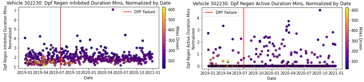
Figure 2: Data Exploration of the Normalized Numeric Attributes
While Figures 1 & 2 show the results for only one truck, this analysis was performed on many of the trucks with no meaningful insights. As a result, we moved onto exploring the trucks’ Diagnostic Trouble Codes.
Diagnostic Trouble Codes
Each DTC has two components, the Suspect Parameter Number (SPN) and the Failure Mode Identifier (FMI), which describe the issue’s nature and severity, respectively.
In addition to SPN codes 3251 and 3720, our sponsor shared with us several DTCs that could be related to DPF failure from SPN and FMI code intuition. However, we were also encouraged to analyze other potential DTCs that could be related to DPF failure. A key heuristic used throughout the analysis was the frequency of specific trouble codes before and after the service date. DTCs that display in rapid succession leading up to a service date and forgo appearance afterwards correspond with failures of particulate filters, as trucks are brought in to be serviced due to the failure of the filters . However, other issues uncommitted to diesel particulate filters are also fixed during the service date. Therefore, analysis alone was not enough to conclude specific DTCs that were related to a DPF failure. To avoid overfitting, we used DTCs where we could see patterns of rapid growth and decay around the service date and our sponsor could corroborate as having some connection related to DPF failure from intuition. Our analysis confirmed some of the DTCs to which our sponsor alerted us like SPN 3251 FMI 0 and SPN 3720 FMI 15 and uncovered new ones such as SPN 3216 FMI 18 that were all used in the model.
There are many different DTCs relating to all parts of the vehicle, including the brakes, transmission, engine, and even the onboard camera. Per our sponsor’s advice, we paid close attention to the occurrences of DTCs with SPN code 3720 and 3251, which measures ash accumulation and pressure built-up in the engine. As seen in Figure 3, their daily occurrences spiked significantly before DPF failure.

Figure 3: Frequencies in occurrences of DTCs with SPN code 3720 and 3251
Data Pre-processing & Extraction
Resetting service dates in the train set
The imbalanced distribution of trucks with and without DPF failure means that there are more daily records for trucks with DPF failure than those without in the train set. The opposite is true for the test set. There are 2,308 daily trip records fourteen days before service dates in the train set – 1,361 and 947 of which belong to trucks with and without DPF failure respectively. On the other hand, there are 731 daily trip records fourteen days before service dates in the test set – 240 and 491 of which belong to trucks with and without DPF failure respectively.
To combat this, we use a simple function that sets the date of service for trucks without DPF failure in the train set to the date of the last record available – rather than the January 1st proxy that Vnomics uses as default. This allows us to extract as many records as possible for trucks without DPF failure in the train set, resulting in a more balanced train set. We have tried to combat the data imbalance at first with Synthetic Minority Oversampling Technique (SMOTE). However, with the windowing process, which we introduced in the latter part of feature engineering, we were able to clear the data set of any data imbalance. Moreover, we were later able to achieve a much higher result without the use of synthetic data to generate new records ensuring the training data is authentic and as close to real-world data as possible while benefitting from a higher accuracy score.
With the reset service dates, there are now 1,035 records of trucks without DPF failure rather than 947, adding 88 more records and creating a more balanced data set.
Feature Engineering
Firstly, we create a new variable, miles_per_gallon. As the name implies, it is the distance in miles that the truck traveled with each gallon of fuel on the day. We calculate it by simply dividing the total distance driven in miles (distance_miles) by the total amount of fuel used (fuel_used_gallon) for the day. If a truck has DPF failure, we can expect its engine to operate inefficiently – leading to a lower miles_per_gallon value.
Secondly, we then drop all unused variables. Foremostly, per our sponsor’s advice, we drop the two inhibit switch variables, dpf_regen_inhibit_switch_not_active_duration_mins and dpf_regen_inhibit_switch_active_duration_mins. Both of these appeared to be junk features with little to no signal. We then drop dpf_regen_not_inhibited_duration_mins and dpf_regen_not_active_duration_mins, while keeping their positive counterparts, dpf_regen_inhibited_duration_mins and dpf_regen_active_duration_mins. Since these two pairs of variables both add up to duration_mins, including both features in each pair offers in a model little to no incremental knowledge and can potentially lead to perfect multicollinearity issues.
Lastly, we normalize the remaining features in minutes except duration_mins – which are dpf_regen_inhibited_duration_mins, dpf_regen_active_duration_mins, dpf_regen_needed_duration_mins, and idle_duration_mins – by duration_mins, as discussed previously.
Data Windowing
Upon scaling the data as described above, we are left with 1,669 records in the train set and 467 records in the test set. Per Professor Anand’s suggestion, we decided to window the record data. The intuition is as followed: issues related to DPF failure are likely to be persistent before the service date, most likely lasting longer than a day. By combining records within a certain time frame into successive windows and thus aggregating such effects, we can better extract useful signals from them.
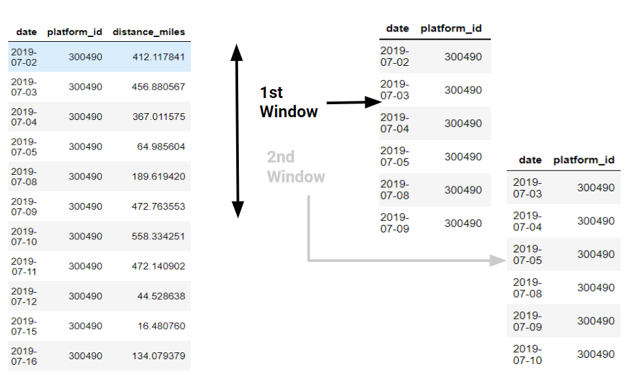
Initially, we planned to use tsfresh – a Python Time Series library – to create rolling windows of the record data. However, because the record data is not uniformly sampled, the output ends up containing a lot of duplicate records. For example, look at the first five rows in Figure 4:

Figure 4: The output of tsfresh’s roll_time_series function on the train record set.
Since we want to keep the training data as authentic as possible, we decided not to impute the data with synthetic records. As such, we must write the windowing functions ourselves. There are two windowing functions, one produces sliding, non-overlapping windows while the other produces moving, overlapping ones.
For example, consider the set of records below. The first function will create a number of windows that intersect at their starts and ends but do not overlap, with a chosen time gap between the start and end date for each truck. The window created will contain all records present between the start and end date. With the default number of windows of two and time gap of seven, it will create a window from 07/02 to 07/09, then another from 07/09 to 07/16.

The second function will instead fit a window, with a chosen time gap between the start and end date for each truck, at each date if possible. From the set of records above, with the default time gap of seven, it will create the same first window from 07/02 to 07/09 as before. However, it will then create a second window from 07/03 to 07/10, a third from 07/04 to 07/11, and up to one last window from 07/09 to 07/16.
Upon creating the windows, we would use tsfresh to extract useful features from each of them – such as the mean, median, and variance of each variable within the window. We also count the occurrences of important DTCs in each window and normalize them by the length of the window. The logic is the same as above for variables measured in minutes besides duration_mins: the produced windows in either method will very likely have varying lengths. Consider a window of length six and another of length four: suppose a DTC occurs on four days in both of them. While the occurrence counts are equal, this DTC is active for four out of six days in the first window, but four out of four days for the last.
Model Building
After performing windowing, we have 951 overlapping windows and 182 non-overlapping windows from records in the train set. On the other hand, we have 267 overlapping windows and 97 non-overlapping windows from the test set.
For our classification, we decide to classify each truck’s windows and aggregate the predictions to get the predictions on each individual truck. All the windows will share the same labels as their trucks: windows of trucks with and without DPF failure are labeled as True and False. If any of a truck’s windows is predicted to be True, that truck is predicted to have a DPF failure.
The distribution of labels for windows of each type is shown in the table below:

Table 1: Distribution of labels for windows.
Our chosen model is Random Forest, implemented by the sklearn library’s method RandomForestClassifier. Random Forest has been proven to be extremely robust to outliers – which some of the records might be – and non-linear interactions between variables. More importantly, besides performance, Random Forest allows us to extract feature importances and examine which features best predict DPF failure.

Table 2: Base Random Forest’s performance with non-overlapping windows

Table 3: Base Random Forest’s performance with overlapping windows
Before fitting the base model, we removed junk variables like window length and performed an F-Test to select only the most relevant half of all variables – leaving us with 36 variables remaining. As shown above, while Random Forest does overfit the training data, its performance is still very admirable on the testing in both cases. Interestingly enough, the performance on predictions of trucks is identical for both overlapping and non-overlapping data. To reduce overfitting, we perform tuning with Optuna.
Trials are scored by Accuracy measured in Stratified 10-Fold Cross-Validation.
Performances and Results

Table 4: Tuned Random Forest’s performance with non-overlapping windows

Table 5: Tuned Random Forest’s performance with overlapping windows
Overall, tuning improves the performance of window predictions for both test sets but has mixed effects on truck predictions. With non-overlapping windows, all metrics for truck predictions on the test set improve except for Recall which drops from 100.00% in Table 2 above to 93.75%. In particular, Accuracy noticeably increases from 75.51% to 79.59%. On the other hand, with overlapping windows, the Accuracy of truck predictions on the test set fails to improve. Only Recall marginally improves from 57.14% to 58.33%, at the cost of F1-Score dropping from 72.73% to 70.00% and Recall significantly dropping from 100.00% to 87.50%. Based on this, we conclude that the tuned Random Forest using non-overlapping data is the best model.
We then examine feature importance, based on this best model. The most critical predictor of DPF failure is the diagnostic code SPN 3720 FMI 15, which measures ash accumulation in DPF. The second most critical predictor is SPN 3216 FMI 18, which measures the number of nitrogen oxides entering the after-treatment system. The fifth most critical predictor is SPN 3251 FMI 0, which measures pressure in the after-treatment system. The longer these DTCs are present in each window, the more exhaust emissions are likely trapped in the DPF – clogging the filter. In particular, SPN 3720 FMI 15 has much greater importance than any other variable, as shown in the plot below. All models – tuned or untuned – recognize it as important.


Figure 8: Confusion Matrices for the best model’s predictions on trucks in the train set (Left) and test set (Right)
The other significant features besides the three DTCs in the graph above can be divided into two groups. The first group of variables deals with the duration of DPF regeneration:
- dpf_regen_inhibited_duration_perc__sum_values: The total percentage of time where regeneration is inhibited in a window
- idle_duration_perc__minimum: The minimum percentage of time where a truck is idle in a window. Higher values suggest extended parked regeneration or even engine failure
- dpf_regen_active_duration_perc__variance: The variance in the percentage of time where regeneration is active in a window
- dpf_regen_inhibited_duration_perc__maximum: The maximum percentage of time where regeneration is inhibited in a window
The second group of variables deals with efficient fuel consumption. The more fuel the engine must burn to operate, the more likely the filter is clogged:
- miles_per_gallon__mean: Mean miles per gallon in a window
- miles_per_gallon__minimum: Minimum miles per gallon in a window
- fuel_used_gallons__sum_values: Total fuel used in gallons in a window
Conclusion & Next Steps
Foremost, the most important indicator of imminent DPF failure is the amount of exhaust emissions in the filter. The more emissions are trapped in the filter, the more likely the DPF will get clogged up and fail. As such, the next step should be to examine other DTCs that indicate the presence of trapped exhaust gasses and similar materials. Besides the diagnostic codes, the duration of time a truck spends in DPF regeneration and its fuel consumption during a time window are also critical predictors of DPF failure.
Lastly, it appears that factors that cause DPF failure are fairly persistent. This is because using overlapping windows, which aggregates these effects a lot more times than non-overlapping windows, fails to improve forecast performance. However, further experimentation on window lengths and periods before the service dates should be conducted (i.e. using records within 30 days before the service dates, with a window length of 14 days) to see if the results with each type of window can be improved.