Team Members
Oliver Annon, Audio and Music Engineering ’26
Raffael Venterea, Audio and Music Engineering ’26
Emma Wang, Audio and Music Engineering ’26
Project Description
Unscheduled downtime due to mechanical issues is an expensive and sometimes dangerous problem. This can range from something as simple as a conveyor belt not running to a serious case, such as a submarine’s life support system failing. The standard answer to this problem is routine maintenance, but this still creates downtime, requires additional manual labor, and may miss faults that can only be noticed during operation. The target of this project was to develop a remote sensor that can detect mechanical failures when they occur and use acoustic cues to predict component lifespans. This would inform technicians which repairs are imperative and reduce unnecessary downtime. Current solutions are expensive and typically reserved for high-end machinery. Developing a budget-friendly option creates an opportunity to deploy this technology to a wide range of systems. To achieve this, a custom mechanical test bench was designed, and an Arduino Nano was loaded with a machine-learning model trained on collected acoustic data to detect faults.
The Mechanical Testbench
Considerations
When drafting the testbench design, the goal was to create a repairable failure environment. This meant that components could be intentionally damaged in a known way and then returned to regular operation after testing concluded.
Four main failure points were selected to emulate common faults in real-world mechanical environments. These were: axle misalignment, rotational unbalance, multiple gear transmission issues, and ball bearing failure. We designed 3 main components: The balanced wheel, bearing housing, and jackplate. Then, pre-fabricated parts were attached to complete the system.
Repeatable trials are critical for conclusive experimental results, so each of these failure points needed to be controllable and repairable. This was achieved for each through the following methods:
- Axle misalignment: Shaft coupling with 2 degrees of freedom and a baseplate with jack screws.
- Rotational unbalance: Balanced wheel with off-center mounting points for weight
- Gear Transmission issues: Miter junction with a swappable set of healthy and damaged gears.
- Bearing Failure: Housing containing slip-fit bearings, one of which can be removed and swapped with a damaged bearing.
In addition to containing these features, the test bench needed to be portable, which meant reducing the size and weight as much as possible, while still maintaining an effective range of capabilities.
Process
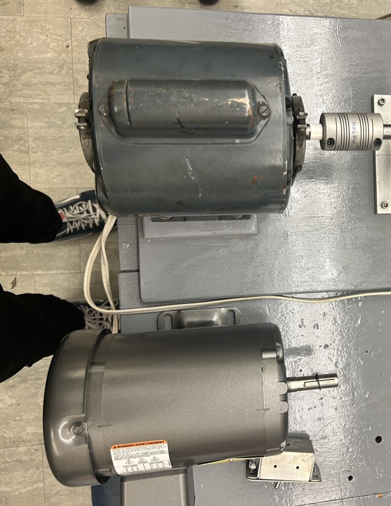
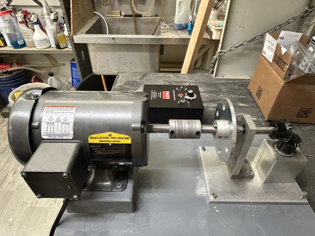
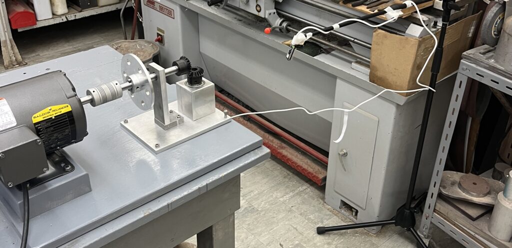
To begin, the initial motor was measured out, and an approximate recreation was modeled. This would later be replaced by a Baldor M3452, pictured at the bottom right. This upgraded the setup from a 1/4 hp single-phase motor to a 3/4 hp three-phase motor, enabling efficient RPM control via a variable-frequency driver (VFD).
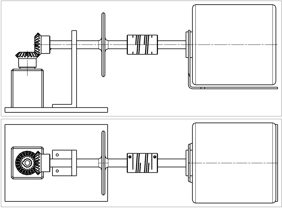
A shaft coupling was then clamped onto the driveshaft of the motor. This coupling allowed for the receiving axle to be tilted up to 2 degrees off-axis. This completed the first adjustable failure point for axle misalignment.
For the second adjustable failure point, a balanced wheel is attached to the receiving axle, halfway between the coupling and the support pillar. Six evenly spaced holes are milled to allow attachment of weights. It is designed with a 5″ diameter to strike a balance between the impact of attached weights on rotational imbalance and the safety of the test bench operator.
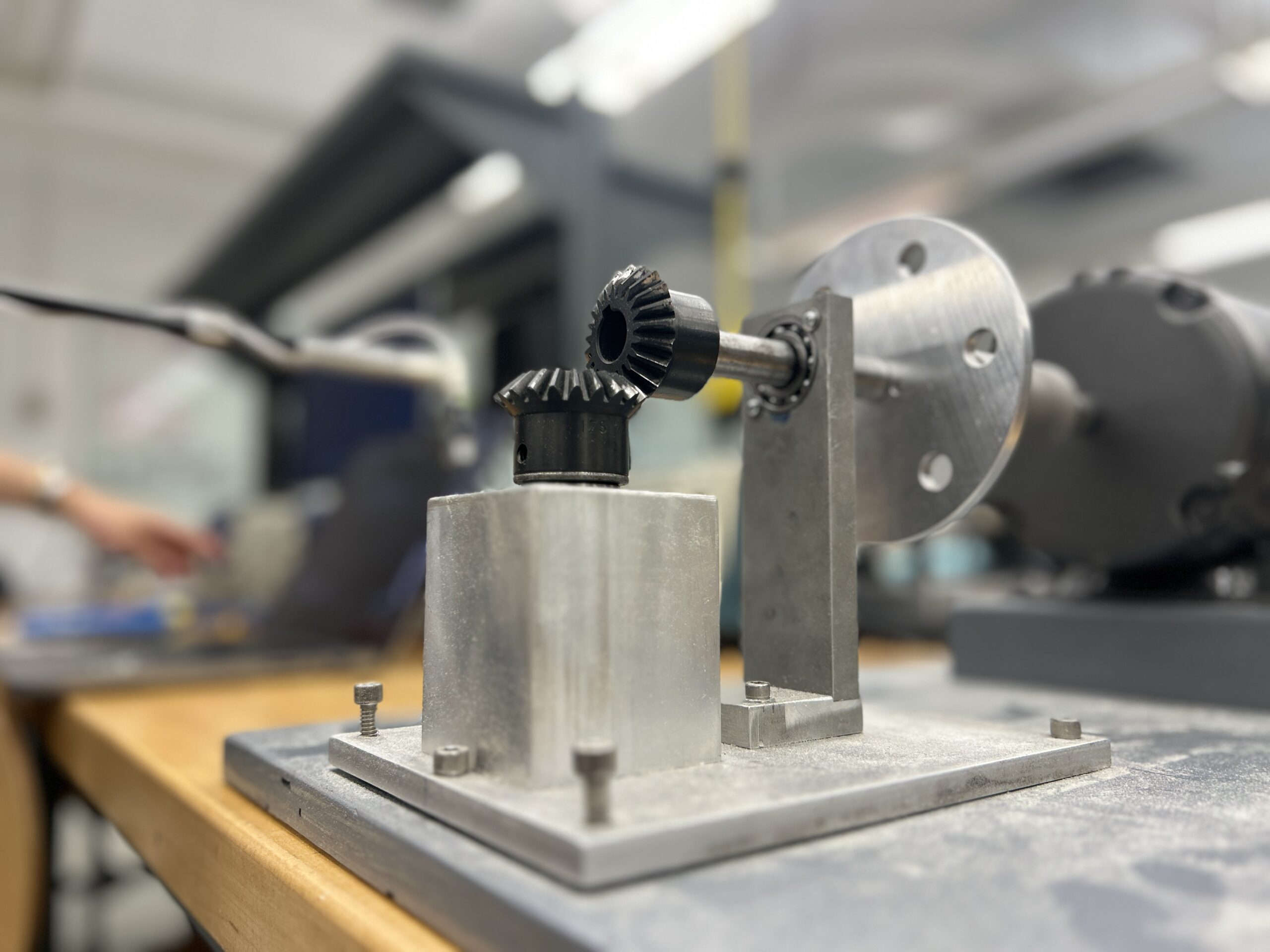
The third and fourth failure points are contained within the gear transmission and bearing housing. Two miter gears provide a transmission from the drive axle to the receiving axle, which is encased in the bearing housing. Slip-fit bearings are installed in the housing, allowing easy removal and replacement of the gears. Four gears were purchased, with three kept original as the healthy set and a fourth intentionally damaged by grinding one of its teeth off. This is how the failure was provided.

The bearing housing is designed to allow removal of the bearings, for which a set was also purchased. Two were kept in their original condition, while a third is planned to have damage applied to it. The receiving gear and axle (sitting vertically) can easily be removed by loosening the set screw on the drive shaft gear (sitting horizontally), sliding it back along the axle, and then lifting the set out of the housing. Pictured left is the test bench running with the receiving gear removed. Two spacers were later added to the receiving axle, below the gear but above the bearing, to ensure solid contact in the gear transmission.
All of these components are mounted to the 8×6″ jackplate. This ensured that all components on the drive axle would tilt at the same angle and place strain only on the shaft coupling. This plate is adjustable via screws on the edge farthest from the motor. The jackplate and motor are then attached to the baseplate, allowing for easy transportation.
Machine Learning Model Design
Arduino Microphone Sensor

https://m.media-amazon.com/images/I/61MC7q9EEVL.AC_SX679.jpg
Our project required deploying a trained machine learning model onto an Arduino Nano 33 BLE Rev 2 sensor – a microcontroller with an onboard PDM microphone and around 256KB of SRAM available for runtime memory [1]. Overall, it has pretty tight memory and compute constraints. However, this board aligns with the project’s broader goal, which is to demonstrate that effective fault detection model can run on such accessible, low-cost hardware rather than only on specialized, high-end equipments. We wanted to find out how much capability we can push out of a compact and multi-functional board like this.
Edge Impulse
The constraints shaped our methodology for model training. In order to extract feature in a way that’s light enough to run on board in real time, as well as fitting the model within the board’s available memory, we chose Edge Impulse as our development platform.
Edge Impulse is a embedded machine learning platform [2]. Instead of streaming sensor data to remote servers for processing and send results back, Edge Impulse models run locally on the device itself. The platform consolidates and simplify the full machine learning workflow – data collection, signal pre-processing, model training and evaluation, and deployment – into a single web-based interface [2]. It’s essentially a pipeline that takes raw input, passes it through processing blocks for feature extraction, then through a learning block that produces the final output.
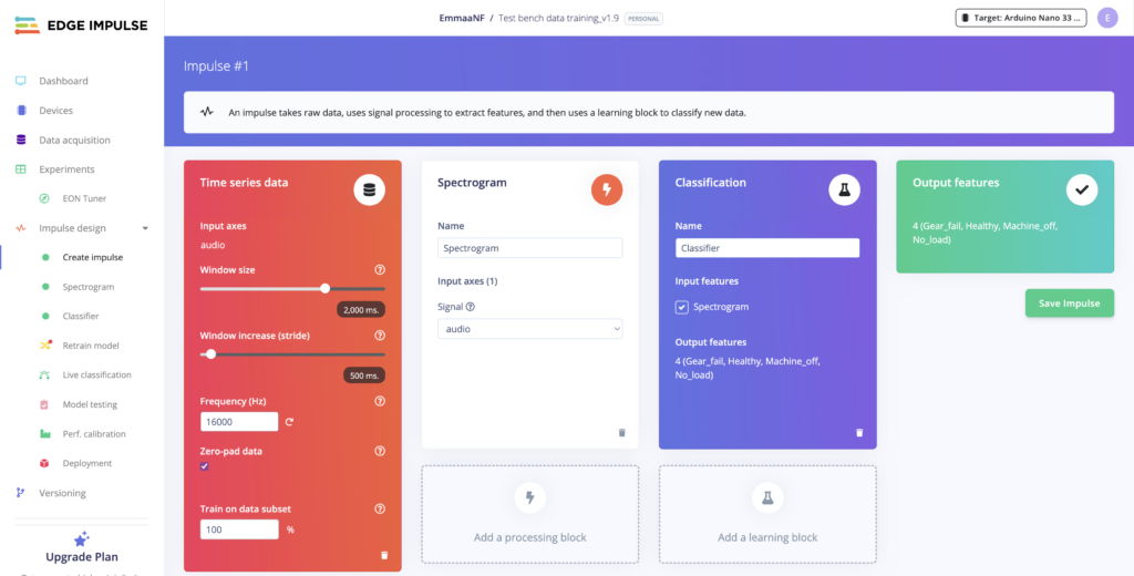
In our case, we configured the learning block to be a classifier of the four machine states: Healthy, Gear_Fail, No_Load, and Machine_Off. Given sufficient clips of audio samples from the test bench to train the model on, the model will learn to output a state that it thinks the input most likely belongs to.
The Processing Blocks – Feature Extraction
Spectrogram
While the model can learn from raw audio waveforms directly, it’s rarely efficient because most of details from one second of audio – which contains thousands of samples – isn’t relevant to distinguishing between different machine states. More importantly, the pattern that would distinguish between healthy and failure states aren’t really visible in the waveform that is in amplitude over time.
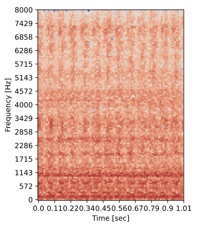
The distinctive features lie in the frequencies that are present in the sound, and spectrogram is essentially a 2D image that shows how those frequencies change over time. With the dimension formed by time on the horizontal axis and frequency on the vertical axis, the color of each pixel shows how much energy is present at that frequency at that moment. Spectrograms turn audio classification into an image recognition problem that suits to convolutional neural networks.
Specifically, spectrogram processing block produces this representation by first slicing the audio into short overlapping windows. Then, within each window, it measures the energy of frequency present in each band, and outputs an image in time-frequency domain. The learning block will treat this image as input.
Audio (MFE)
The Audio (MFE) processing block is essentially a spectrogram block that applies Mel-scale, a scale that maps physical frequencies to align with human pitch perception. This means when grouping the frequency into bands, there is more resolution at lower frequencies. While the Mel scale was developed for speech recognition, its emphasis on lower frequencies also suits mechanical fault detection, as many fault features may appear in the low mid frequency range.
The Learning Block – Classification
A neural network consists of several layers, each layer made up of number of neurons. The system will randomly initialize the weights of the connections between two adjacent layers of neurons. When given a training data as input, the network passes the value through its layers, with each layer adjusting the input based on the current weights. The final layer outputs a probability score for how likely the input is belong to a certain category.
The training works by comparing this output to the correct answer, and, based on that, adjust the weights of the connections between the neurons int he layers, so that future predictions are closer to truth. The process repeats over many inputs and passes using the input data until the network is able to produce reliable prediction on input it never seen before.
The Air Compressor Dataset
Preparation for Data Collection
Parallel to the design and manufacturing process of the workbench, our team started developing understanding and methodology of data collection based on an existing dataset of an air compressor. The goal at this stage was to surface roadblocks early, so we could identify the external variables our methodology would need to account for during real data collection process.
Some recognized factors are as follows:
- Environment – Background noise varies across spaces.
- Recording distance – Microphone distance to source affects signal amplitude.
- Source directionality – Source direction relative to the microphone affects signal frequency profile.
- Model robustness – Model may overfits to remember specific recording samples.
Methodology and Data Pre-Processing
The air compressor dataset includes a variety of machine fault categories, each includes around 250 samples. Our team aimed to design methodologies that avoid the influences by the aforementioned factors as much as possible. To hold environment constant, we connected short data samples back into a long continuous audio for it to be played back and rerecorded through a pair of stereo speakers in the target environment where we would also be testing in. To further eliminate volume as an influential factor as a result of inconsistent recording distance, we performed data normalization through MATLAB.
To test how to promote model robustness, we used two approaches. First, we recorded the sources with low level of white noise playing alongside, which means the noise was captured in the same acoustic environment as the source. Second, we recorded clean sources and added white noise digitally during training as a data augmentation step. Comparing the two strategies helped us understand that while the first approach does introduce variability with acoustical consistency to the data, digital noise augmentation is more constant and controlled spatially.
Model Training
Training Confusion Matrix
Proceeding to the feature extraction stage, we configured Audio MFE block. We started from Edge Impulse’s auto tuned parameters (frame length 25 ms, stride 10 ms, FFT length 512, 41 filters). These values provided balance between frequency and time resolution for general audio classification. In the validation run, these parameter settings produced strong accuracy reflected through the training confusion matrix in early experiments. So, we kept these parameters and were ready to use them as a start off points for the official test bench model training.
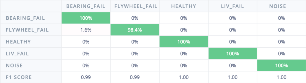
Testing Confusion Matrix
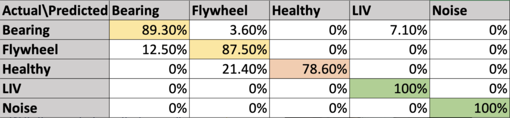
When we tested the model on a new set of testing data that the model has never seen, the accuracy dropped from roughly 99% to about 78-89%. This informed us about the accuracy gap between training and testing stage that strong accuracy doesn’t necessarily reflect how a model behave on testing in real-world environment. This shaped how we approached test bench data collection and model training.
The Test Bench Dataset
Data Collection
As soon as the Test Bench was completed data collection began. Considering the aforementioned variables when capturing data we applied the following to our procedure of capturing audio from the Test Bench.
- Multi-Directional Recordings
- Variable Recording Spaces
- Multiple Takes For Each Machine State
- Variable Frequency Driver (VFD) Consistency
The machine was recorded from three different directions to help improve our models ability to identify new data. This robustness in our raw data was designed to help the model gain more information about the machine and thus have more accurate predictions. Additionally, the machine was moved to and recorded in three different locations. These locations varied in negligible amounts of background noise (HVAC vs Non HVAC) and room acoustics (Carpet vs Stone Walls) but were still considered as a means to help improve the models accuracy. Further more, every time the machine was recorded on a new take the machine was disassembled and reassembled into as proper of a state as possible. This allowed us to capture multiple takes of the same machine state from the same position, while still having the new data provide something more to the data set as a whole. Finally, another variable that had to be kept in check was the speed of the motor. To keep this as consistent as possible we had our machine operator turn the Variable Frequency Driver (VFD) to the same position during operation. Regardless of room, state or recording position the VFD was always set to 50%. This was an attempt to remove any audible changes in the motor as it was not a component we were considering for fault.
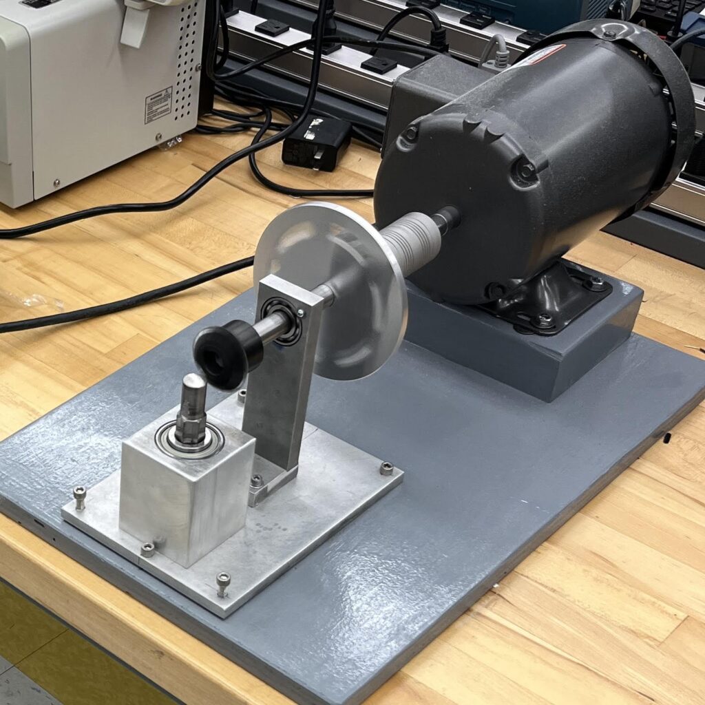
Below you can see our machine set up for recording in one of our recording spaces.

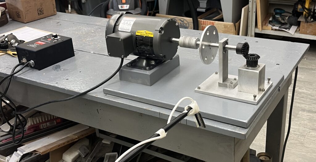
The recording positions here all place the microphone one foot away from the machine at varied angles. With position 1 at 0o or 360o, Position 2 at 90o, and Position 3 at 180o we believed that our recordings would allow us to observe the machine at any point along this 180o arc.
Model Training
With our new data we were able to make a variety of different models that considered both model hyperparameters and different model architectures. However, our search to find these optimal hyperparameters and model architectures was limited by our project’s scope, as the need to hire an engineer to design a monitoring system would be an unnecessary expense for a small businesses. Thus, we limited ourselves to editing our models solely via Edge Impulse. [2] This did allow us to change windowing parameters for our feature extractor, number of training cycles, learning rate, type of feature extractor, data augmentation, and learning processes. (Classification vs Anomaly Detection )
With all this at our disposal we first made a simplified model that was tasked with distinguishing between two different machine states. This model preformed well after being trained on a set of data obtained from a single recording session. From here more data was collected and more complex models were developed to include four different machine states in total. A limitation that we encountered during testing was the amount usable memory on our Arduino Board. [1] When developing different models we were not able to deploy more complex feature extractors or learning architectures. This forced us to only consider a classifier that either had a spectrogram or a Mel-Frequency feature extractor.
Inferencing video
Result
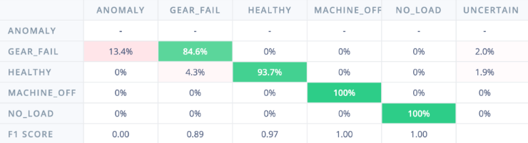
After varying the aforementioned variables in Edge Impulse and with their respective verification sessions we were able to develop a model with the following Verification Confusion Matrix. While this model had the best performance across the largest number of machine states, it was still not accurate enough for us to consider the model a success.
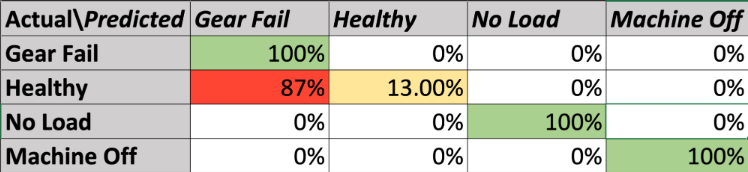
The model itself is a 1D Convolutional Neural Network with 2 layers. It uses a Mel-Frequency feature extractor and classification learning with four labels. While this model isn’t accurate enough to consider a success, there are several points worth mentioning. Every faulty state – gear fail, no load and machine off – was correctly identified 100% of the time. Like the previous air compressor model, the test bench model never classified a faulty machine as healthy. However, the remaining problem is that the model misclassified 87% of healthy samples as gear fail. This means the model has not learnt to separate gear fail and healthy cleanly, and the inspection cost on false alarms might be too high to deploy in a real world setting.
Discussion
While we did not create the budget friendly ease of access product that we wanted, we still collected an extensive data base and explored the limits of Edge Impulse on a Nano 33 BLE Sense Rev2. [2][1] Furthermore, our findings suggest to us that either a multi-model or multi-perspective implementation of the aforementioned methods of machine observance may be successful.
A Multi-Model implementation would be an Edge Impulse Model that is able to run both a Classifier and and an Anomaly Detector to interpret new audio in parallel.[2] This type of model would not only allow for known fault classification but also for detecting when the machine is in an undiagnosed state. As mentioned a Nano 33 is not a sufficient machine and thus we were not able to get a verification matrix for this specific model. We did, however, produce a training matrix.
A Multi-Perspective implementation would include the use of more than more microphone during inferencing. During, our testing we found that specific model’s behavior would change as it was moved around the machine. Incorporating multiple perspectives during inferencing with the same model could help that model to have more accurate inferencing.